9.3: Project Decision Metrics: Net Present Value

Last updated
Save as PDF

Page ID: 47806

$ \newcommand{\vecs}[1]{\overset { \scriptstyle \rightharpoonup} {\mathbf{#1}} } $ $ \newcommand{\vecd}[1]{\overset{-\!-\!\rightharpoonup}{\vphantom{a}\smash {#1}}} $$\newcommand{\id}{\mathrm{id}}$ $ \newcommand{\Span}{\mathrm{span}}$ $ \newcommand{\kernel}{\mathrm{null}\,}$ $ \newcommand{\range}{\mathrm{range}\,}$ $ \newcommand{\RealPart}{\mathrm{Re}}$ $ \newcommand{\ImaginaryPart}{\mathrm{Im}}$ $ \newcommand{\Argument}{\mathrm{Arg}}$ $ \newcommand{\norm}[1]{\| #1 \|}$ $ \newcommand{\inner}[2]{\langle #1, #2 \rangle}$ $ \newcommand{\Span}{\mathrm{span}}$ $\newcommand{\id}{\mathrm{id}}$ $ \newcommand{\Span}{\mathrm{span}}$ $ \newcommand{\kernel}{\mathrm{null}\,}$ $ \newcommand{\range}{\mathrm{range}\,}$ $ \newcommand{\RealPart}{\mathrm{Re}}$ $ \newcommand{\ImaginaryPart}{\mathrm{Im}}$ $ \newcommand{\Argument}{\mathrm{Arg}}$ $ \newcommand{\norm}[1]{\| #1 \|}$ $ \newcommand{\inner}[2]{\langle #1, #2 \rangle}$ $ \newcommand{\Span}{\mathrm{span}}$$\newcommand{\AA}{\unicode[.8,0]{x212B}}$

Project Decision Metrics: Net Present Value

Suppose that you were an electric utility considering two potential generation investment opportunities: A natural gas fired generator with a capital cost of 600 dollars per kW and operating costs of 50 dollars per MWh, or a wind farm with a capital cost of 1,200 dollars per kW and operating costs of 5 dollars per MWh. For the purposes of this example, assume that either power plant could meet the same reliability goals that your utility had. But your regulator wants you to minimize economic costs to consumers. Which should you pick?

This is a difficult choice because it involves tradeoffs over time. The natural gas generator has a low up-front cost but a higher operating cost. The wind generator has a higher up-front cost but a very low operating cost, because fuel from the wind is free (at the margin). This tradeoff is shown visually in Figure 9.1, for a 1 MW natural gas and wind power plant — for the sake of comparison, we assume that each of the plants operates 30% of the time, so each produces 1 MW × 8,760 × 0.3 = 2,628 MWh per year.

This 30% figure is called the capacity factor, and it measures how much electricity a power plant produces in a year versus how much it could produce each year if it operated all the time at 100% capacity.

$\text { Capacity Factor }=(\text { Annual Production }) \div(\text { Capacity } \times 8,760 \text { hours per year) }$.

$Figure \text { } 9.1$ illustrates the tradeoff but doesn't say much about which decision you should make. Part of the problem is that by investing in the wind turbine, you are accepting a high cost right now in exchange for a stream of operating cost savings in the future. Is this stream of operating cost savings worth it?

One of the most frequently-used metrics to compare projects with different capital and operating cost streams is the net present value, which incorporates the present discounted value of all project costs and revenues.

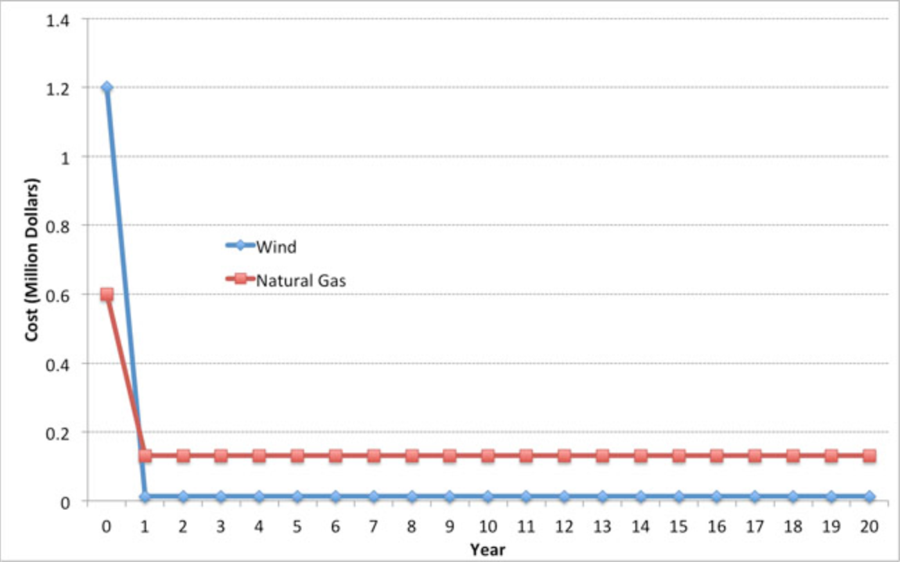
$Figure \text { } 9.1$: Capital and operating costs for a 1 MW natural gas and wind power plants over a 20-year operating horizon.

The net present value $(NPV)$ is defined by two terms: the present discounted value of costs and the present discounted value of revenues. If we let $B_{t}$ be the (undiscounted) revenues (benefits) of some project during year $t$ and we let $C_{t}$ be the (undiscounted) costs of the same project during year $t$, then we can calculate the $NPV$ as follows:

$\begin{array}{l}
\text { Present discounted benefits }=P D B=\sum_{t=0}^{T} \frac{B_{t}}{(1+r)^{t}} \\
\text { Present discounted costs }=P D C=\sum_{t=0}^{T} \frac{C_{t}}{(1+r)^{t}} / p> \\
\text { Net present value }=N P V=P D B-P D C=\sum_{t=0}^{T} \frac{\left(B_{t}-C_{t}\right)}{(1+r)^{t}}
\end{array}$

In the equations, $T$ is the time horizon for the project and $r$ is the discount rate. If the net present value of a project is greater than zero, then the project is said to break even or be "feasible" in present discounted value terms. If you are in a position where you are evaluating multiple alternatives, you would normally want to choose the alternative with the highest net present value.

Sometimes, we will be interested in the net present value of a project as of some year prior to $T$. We will call this the "Cumulative NPV" as of year $X$. Mathematically, this is defined as: $\text { Cumulative NPV }=\sum_{t=0}^{X} \frac{\left(B_{t}-C_{t}\right)}{(1+r)^{t}}$

Where $X$ is some number smaller than $T$.

To illustrate, let's go back to one of our examples from earlier in this lesson. Our wind power plant had a capital cost of $1.2 million and annual operations costs of $13,140. Suppose that it had annual revenues of $100,000 and faced a discount rate of 10% per year. Each year, it thus has annual profits of $86,140.

Assuming that all of the capital costs were incurred in Year 0 and the plant began operating in Year 1, the present discounted value of each of the first three years of operation would be:

$\begin{aligned}
&P V(O)=-\$ 1.2 \text { million (this is just the capital cost, note that this is a negative number) }\\
&P V(1)=\$ 86,140 \div(1.1)^{1}=\$ 78,963.64\\
&P V(2)=\$ 86,140 \div(1.1)^{2}=\$ 71,785,12\\
&P V(3)=\$ 86,140 \div(1.1)^{3}=\$ 65,259.20
\end{aligned}$

The Cumulative $NPV$ for the first three years would be:

$\begin{array}{l}
\text { Cumulative } N P V(0)=P V(0)-\$ 1.2 \text { million } \\
\text { Cumulative } N P V(1)=P V(0)+P V(1)=-\$ 1.12 \text { million } \\
\text { Cumulative } N P V(1)=P V(0)+P V(1)+P V(2)=-\$ 1.05 \text { million } \\
\text { Cumulative } N P V(1)=P V(0)+P V(1)+P V(2)+P V(3)=-\$ 983,992
\end{array}$

Calculating $NPV$ is reasonably straightforward in a spreadsheet program such as Excel. eare two functions in Excel, $PV$ and $NPV$, that will calculate net present value for you. The difference between the $PV$ and $NPV$ functions is that the $PV$ function assumes that you have the same profits in each period (as in our example above), while the $NPV$ function does not make this assumption.

The video below shows an example of evaluating $NPV$ using Excel. The example in the video is our natural gas plant from the previous lesson. Registered students can access the Excel file discussed in the video in Canvas.

Video: NPV Example Video (15:19)

There are two special cases where calculating the $NPV$ is especially simple - the "annuity" and the "perpetuity." When a project's annual cash flow is the same in each year, not unlike a fixed-rate mortgage, we refer to this type of project as having an annuity structure. In this case, because the cash flow is the same each year, the summation term in the $NPV$ can be greatly simplified. The formula for the present value of an annuity is shown below; if you are interested you can find the derivation in the reading accompanying this lesson.

$\text { Present Value of Annuity }=a \times\left(\frac{(1+r)^{T}-1}{r \times(1+r)^{T}}\right)$

where $a$ is the annual cash flow. To illustrate this, let's calculate the present value of the wind power plant over a three year operating time horizon ($T=3$), using the annuity formula. One of the tricks here is that you need to take the Year 0 cash flow (the 1.2 million dollars capital cost) outside of the formula.

$\text { Present Value }=-\$ 1.2 \text { million }+86,140 \times\left(\frac{(1.1)^{3}-1}{0.1 \times(1.1)^{3}}\right)=-\$ 983,992$, which is just what we got using the $NPV$ formula.

If an annuity involves identical payments over a long period of time (tens of decades, for example), we can approximate the $NPV$ of the annuity using an extremely simple formula called a perpetuity. If we take the annuity formula and let $T$ get really really large (tending towards infinity) then the "-1" term from the numerator becomes meaningless relative to the $(1+r)^{T}$ term, and the present value becomes:

$\text { Present value of a perpetuity }=a / r$.

As a rule of thumb, if the annuity lasts longer than 30 years, you can probably approximate the present value reasonably well using the perpetuity formula.