18.2: MIMO Loop Shaping

Let us now revisit the above example in the MIMO setting. The example will require the following facts about singular values, so we ask you to confirm these facts for yourself before proceeding:

1. \(\sigma_{\max }(A B) \leq \sigma_{\max }(A) \sigma_{\max }(B)\), and
2. If \(\sigma_{\max }(C D)<1 \text { then } \sigma_{\max }(C)<\frac{1}{\sigma_{\min }(D)}\) assuming \(D\) is invertible

The first statement follows from the fact that \(\sigma_{\max }\) is the induced 2-norm, and therefore submultiplicative. To prove the second, apply the first with \(A = CD\) and \(B = D^{-1}\).)

Example 18.2: MIMO Disturbance Rejection and Weighted Sensitivity

The set-up and formulation for the MIMO case are the same as in the SISO example, with the obvious replacements of SISO subsystems by MIMO subsystems. One again arrives at the equation (18.5). However, the inference from this equation in the MIMO case is no longer (18.6) and (18.7), but rather

\[\sigma_{\max }\left[(I+P(j \omega) K(j \omega))^{-1}\right] \leq \gamma \frac{1}{\sigma_{\min }[W(j \omega)]}\nonumber\]

This leads us to the singular value plot shown in Figure 18.4, which is the natural extension of the plot we had in the SISO example.

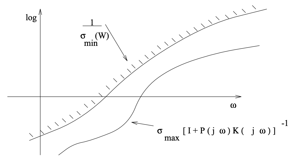
Figure \(\PageIndex{1}\): Singular value plot for a MIMO system

With the insight provided by the above example, we can formulate a variety of MIMO performance problems in terms of appropriate weighting operators. Alternatively, having seen what sorts of modifications of the SISO statements are needed for the MIMO case, we can actually describe various MIMO control tasks in a language that is closer to that of classical SISO control, and this is what we do in the rest of this lecture. We shall return to the explicit use of weighting functions in later lectures.

Typical Closed-Loop Performance Constraints

Typically in control systems the disturbances d have frequency content that is concentrated in the low-frequency range. Therefore, in order to attenuate the effects of disturbances on the output, we require that \(\sigma_{\max }(S(j \omega))\) be small in the range of frequencies where the disturbances are active, say \(0 \leq \omega \leq \omega_{sy}\). On the other hand, typically the noise input \(n\) has frequency content that is concentrated in the high-frequency range. Therefore, in order to attenuate the effect of \(n\) on the output we require that \(\sigma_{\max }(T(j \omega))\) be small over a frequency range of the form \(\omega \geq \omega_{t y}\). The controller \(K\) should also enable the closed-loop system to track reference inputs \(r\) that are typically concentrated in the low frequency range, for example in the interval \(0 \leq \omega \leq \omega_{r}\). This objective requires that \(T(j \omega) \approx I\) for all \(\omega\) in the interval \(0 \leq \omega \leq \omega_{r}\). This requirement can be restated as

\[\begin{array}{l}
\sigma_{\max }(T(j \omega)) \approx 1 \\
\sigma_{\min }(T(j \omega)) \approx 1
\end{array}\nonumber\]

in the frequency range \(0 \leq \omega \leq \omega_{r}\).

The control signals must also generally be kept as small as possible in the presence of both disturbances \(d\) and measurement noise n. It is easy to see that

\[u=(I+K P)^{-1} K r-(I+K P)^{-1} K(d+n)\nonumber\]

Therefore, in order to keep the control signal small, we must make sure that

\[\sigma_{\max }\left((I+K(j \omega) P(j \omega))^{-1} K(j \omega)\right)\nonumber\]

remains small in the frequency range where disturbances and/or measurement errors are effective. We can summarize these design requirements in the following table:

Design Requirement	Closed-Loop Condition	Frequency Range
Sensitivity to Disturbances	\(\sigma_{\max }\left((I+P(j \omega) K(j \omega))^{-1}\right) \approx 0\)	Low frequency \(0 \leq \omega \leq \omega_{s y}\)
Noise Propagation Attenuation	\(\sigma_{\max }\left((I+P(j \omega) K(j \omega))^{-1} P(j \omega) K(j \omega)\right) \approx 0\)	High Frequency \(\omega \geq \omega_{t y}\)
Tracking of Reference Signals	\(\begin{array}{l} \sigma_{\max }\left((I+P(j \omega) K(j \omega))^{-1} P(j \omega) K(j \omega)\right) \approx 1 \\ \sigma_{\min }\left((I+P(j \omega) K(j \omega))^{-1} P(j \omega) K(j \omega)\right) \approx 1 \end{array}\)	Low frequency \(0 \leq \omega \leq \omega_{r}\)
Low Control Energy	\(\sigma_{\max }\left((I+K(j \omega) P(j \omega))^{-1} K(j \omega)\right) \approx 0\)	Frequencies where \(d\) and \(n\) are dominant

Translation to Open-Loop Constraints

Now let us relate the closed-loop requirements that are summarized in the preceding table to open-loop conditions, i.e., conditions on the singular values of the loop gain operator \(P K\). The first design requirement is that \(\sigma_{\max }\left((I+P K)^{-1}\right)\) be small in the frequency range \(0 \leq \omega \leq \omega_{s y}\). The relation

\[\sigma_{\max }\left((I+P(j \omega) K(j \omega))^{-1}\right)=\frac{1}{\sigma_{\min }(I+P(j \omega) K(j \omega))}\nonumber\]

implies that if \(\sigma_{\min }(P(j \omega) K(j \omega))>>1\) then

\[\sigma_{\max }\left((I+P(j \omega) K(j \omega))^{-1}\right) \approx \frac{1}{\sigma_{\min }(P(j \omega) K(j \omega))} \ \tag{18.8}\]

Therefore, if \(\sigma_{\min }(P(j \omega) K(j \omega))>>1\) for all \(\omega\) in the interval \(\left[0, \omega_{s y}\right]\), then \(\sigma_{\max }\left(I+(P(j \omega) K(j \omega))^{-1}\right)\) will be small in that interval.

For noise attenuation, consider

\[\begin{aligned}
\sigma_{\max }(T(j \omega)) &=\sigma_{\max }\left(I-(I+P(j \omega) K(j \omega))^{-1}\right) \\
&=\sigma_{\max }\left(\left(I+(P(j \omega) K(j \omega))^{-1}\right)^{-1}\right) \\
&=\frac{1}{\sigma_{\min }\left(I+(P(j \omega) K(j \omega))^{-1}\right)}
\end{aligned}\nonumber\]

Therefore, for the frequency range \(\omega \geq \omega_{t y}\) we require that \(\sigma_{\min }\left(I+(P(j \omega) K(j \omega))^{-1}\right)\) be as large as possible. This can be guaranteed if we make \(\sigma_{\min }\left(I+(P(j \omega) K(j \omega))^{-1}\right)\) as large as possible or equivalently by making \(\sigma_{\max }(P(j \omega) K(j \omega))\) as small as possible.

The tracking objective can be achieved if we ensure that

\[\begin{aligned}
\sigma_{\max }\left((I+P(j \omega) K(j \omega))^{-1} P(j \omega) K(j \omega)\right) & \approx 1 \\
\sigma_{\min }\left((I+P(j \omega) K(j \omega))^{-1} P(j \omega) K(j \omega)\right) & \approx 1
\end{aligned}\nonumber\]

over the frequency interval [\(0, \omega_{r}\) ]. Since

\[I-(I+P(j \omega) K(j \omega))^{-1}=(I+P(j \omega) K(j \omega))^{-1} P(j \omega) K(j \omega)\nonumber\]

the tracking objective can be achieved if we require \((I+P(j \omega) K(j \omega))^{-1}\) to be close to zero on the frequency range [\(0, \omega_{r}\) ], that is \(\sigma_{\max }\left((I+P(j \omega) K(j \omega))^{-1}\right)\) to be small in that interval. Equivalently, we may require \(\sigma_{\min }\left((I+P(j \omega) K(j \omega))\right)\) to be as large as possible on the interval [\(0, \omega_{r}\) ]. This can be ensured if we require that \(\sigma_{\min }(P(j \omega) K(j \omega))\) be as large as possible over the frequency range [\(0, \omega_{r}\) ].

The constraint of small control energy leads to the condition that \(\left.\sigma_{\max }((I+K(j \omega)) P(j \omega))^{-1} K(j \omega)\right)\) be made as small as possible. However, we have

\[\begin{aligned}
\sigma_{\max }\left((I+K(j \omega) P(j \omega))^{-1} K(j \omega)\right) & \leq \sigma_{\max }\left((I+K(j \omega) P(j \omega))^{-1}\right) \sigma_{\max }(K(j \omega)) \\
&=\frac{\sigma_{\max }(K(j \omega))}{\sigma_{\min }(I+K(j \omega) P(j \omega))}
\end{aligned} \ \tag{18.9}\]

Note that

\[\begin{aligned}
\sigma_{\min }(I+K(j \omega) P(j \omega)) & \leq \sigma_{\max }(I+K(j \omega) P(j \omega)) \\
& \leq 1+\sigma_{\max }(P(j \omega)) \sigma_{\max }(K(j \omega))
\end{aligned}\nonumber\]

so

\[\begin{aligned}
\frac{\sigma_{\max }(K(j \omega))}{\sigma_{\min }(I+K(j \omega) P(j \omega))} & \geq \frac{\sigma_{\max }(K(j \omega))}{1+\sigma_{\max }(P(j \omega)) \sigma_{\max }(K(j \omega))} \\
&=\frac{1}{\frac{1}{\sigma_{\max }(K(j \omega)}+\sigma_{\max }(P(j \omega))}
\end{aligned}\nonumber\]

Therefore, we can minimize the right hand side of equation 18.9 only if we make

\[\frac{1}{\sigma_{\max }(K(j \omega))}+\sigma_{\max }(P(j \omega))\nonumber\]

large in the ranges of frequencies where \(d\) and/or \(n\) are dominant. For example, if \(\sigma_{\max }(P(j \omega))\) is small at a certain set of frequencies of interest then necessarily \(\sigma_{\max }(K(j \omega))\) must also be small on that set. Clearly this condition is not necessary or sufficient to make

\[\sigma_{\max }\left((I+K(j \omega) P(j \omega))^{-1} K(j \omega)\right)\]

small. It only applies to the upper bound of \(\sigma_{\max }\left((I+K(j \omega) P(j \omega))^{-1} K(j \omega)\right)\), which is given by

\[\frac{\sigma_{\max }(K(j \omega))}{\sigma_{\min }(I+K(j \omega) P(j \omega))}\nonumber\]

and it is only necessary for the upper bound to be small.

The following table summarizes our discussion above on open-loop requirements

Design Requirement	Closed-Loop Condition	Frequency Range
Sensitivity to Disturbances	\(\sigma_{\min }(P(j \omega) K(j \omega)) \text { large }\)	Low frequency \(0 \leq \omega \leq \omega_{s y}\)
Noise Propagation Attenuation	\(\sigma_{\max }(P(j \omega) K(j \omega)) \text { small }\)	High Frequency \(\omega \geq \omega_{t y}\)
Tracking of Reference Signals	\(\sigma_{\min }(P(j \omega) K(j \omega)) \text { large }\)	Low frequency \(0 \leq \omega \leq \omega_{r}\)
Low Control Energy	\(\sigma_{\max }(K(j \omega)) \text { small }\)	Frequencies where \(\sigma_{\max }(P(j \omega))\) is not large enough

Figure 18.6 illustrates the open-loop conditions that we have formulated. Note that in this plot the minimum passband open-loop gain is bounded by \(\sigma_{\min }[P(j \omega) K(j \omega)]\), and the maximum stopband open loop gain bounded by \(\sigma_{\max }[P(j \omega) K(j \omega)]\).

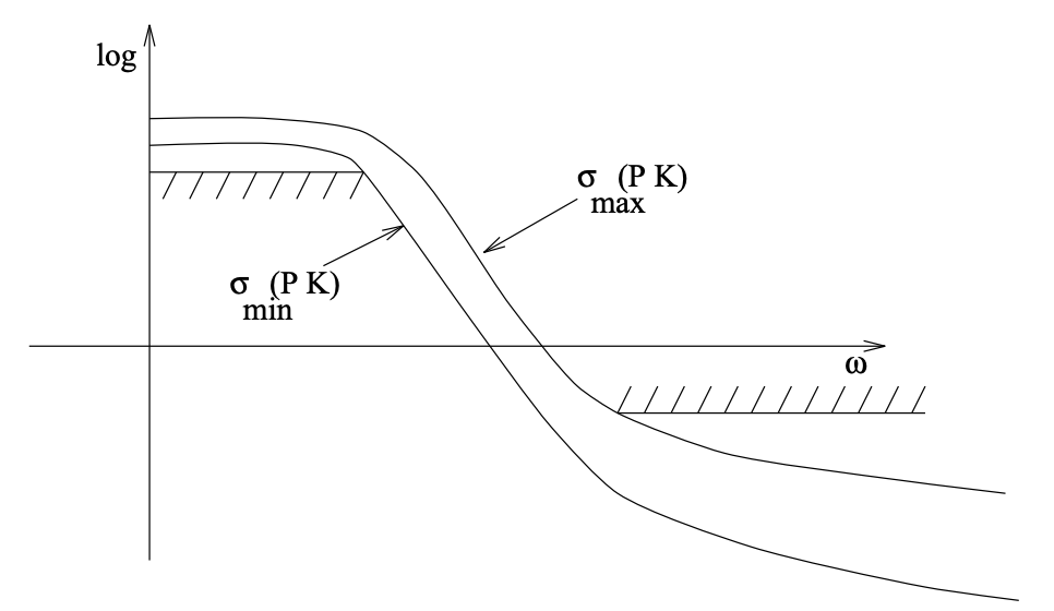
Figure \(\PageIndex{2}\): Singular value bounds for the open loop gain, \(P(j \omega) K(j \omega)\).