1.2: An Industrial Application of Simulation

In order to better understand what simulation is and what problems it can be used to address, consider the following industrial application, which can was used to validate the future state of a plant expansion (Standridge and Heltne, 2000). A particular plant is concerned about the capital resources needed to load and ship rail cars in a timely fashion. A major capital investment in the plant will be made but the chance for future major expansions is minimal. Thus, all additional loading facilities, called load spots, needed for the foreseeable future must be built at the current time and must be justified based on product demand forecasts.

Each product can be loaded only at specific load spots. A load spot may be able to load more than one product. However, it is not feasible to load all products on all load spots. Cleverly assigning products to load spots may reduce the number of new load spots needed. Furthermore, maintenance of loading equipment is required. Thus, a load spot is not available every day.

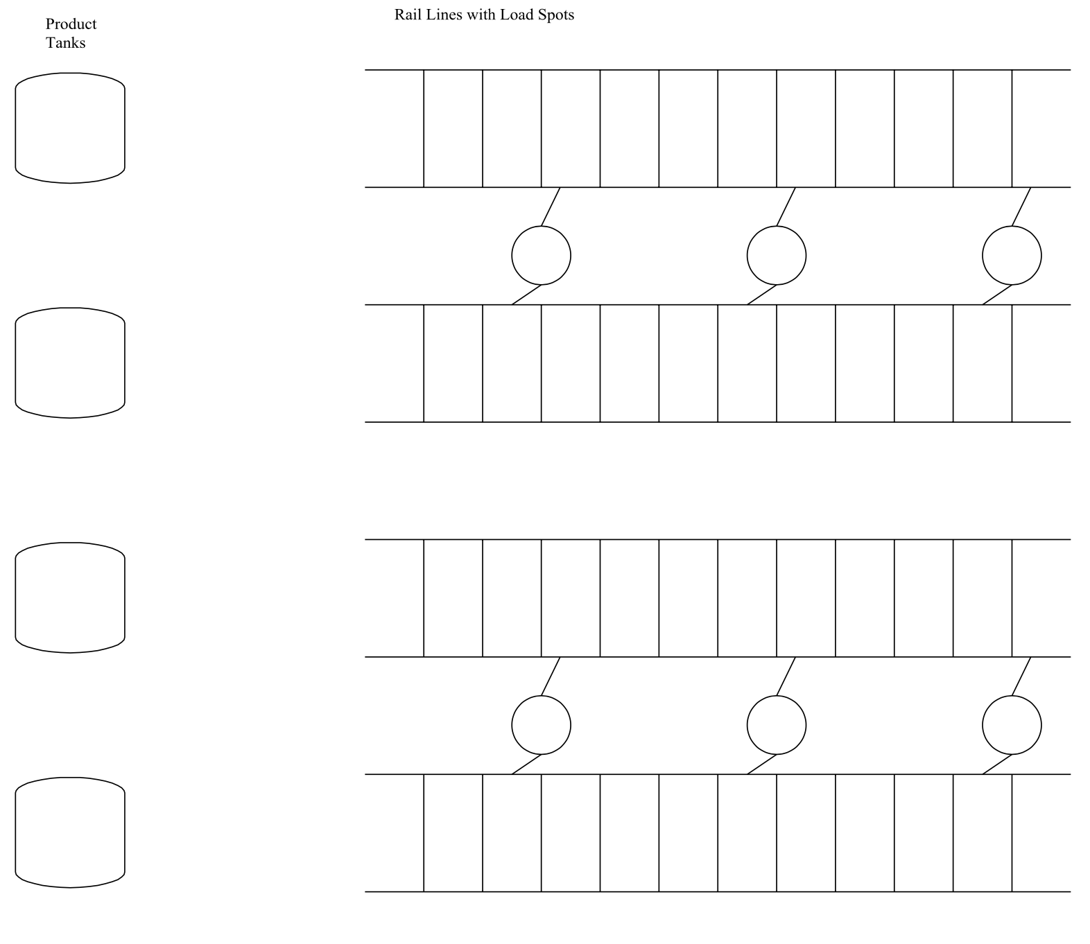
The structure of the product storage and loading portion of the plant is shown in Figure 1-1. Products are stored in tanks with each tank dedicated to a particular product. Tanks are connected with piping to one or more load spots that serve one or two rail lines for loading. These numerous connections are not shown.

The primary measure of system performance is the percent of shipments made on time. The number of late shipments and the number of days each is late are also of interest. Shipping patterns are important so the number of pounds shipped each day for each product must be recorded. The utilization of each load spot must be monitored.

Figure 1-1: Industrial Simulation Application Example

The plant must lease rail cars to ship product to customers. Different products may require different types of rail cars, so the size of multiple rail car fleets must be estimated. In addition, the size of the plant rail yard must be determined as a function of the number of rail cars it must hold.

The model must account for customer demand for each product. Monthly demand ranges from 80% to 120% of its expected value. The expected demand for some products varies by month. In addition, each load spot must be defined by its capacity in rail cars loaded per day as well as the products it can load. Rail car travel times to customers from the plant and from the customer to the plant as well as rail car residence time at the customer site must be considered. Rail car maintenance specifications must be included.

Model logic is as follows. Each day the number of rail cars to ship is determined for each product. A rail car of the proper type waiting at the plant is assigned to the shipment. If no such rail car exists, the model simply creates a new one and the fleet size is increased by one.

Product loading of each rail car is assigned to a load spot. Load spots that can load the product are searched in order of least utilized first until an available load spot is assigned. A load spot may have been previously assigned loading tasks up to its capacity or may be in maintenance and unavailable for loading. Note that searching the load spots in this order tends to balance load spot utilization. The car is loaded and waits for the daily outbound train to leave the plant. The rail car proceeds to the customer, remains at the customer site until it is unloaded, and then returns to the plant. Maintenance is performed on the car if needed.

Analysts formulate alternatives by changing the assignment of products to load spots, the number of load spots available, and the demand for each product. These alternatives are based, in part, on model results previously obtained.

This example shows some of the primary benefits and unique features of simulation. Unique system characteristics, such as the assignment of particular products to particular load spots, can be incorporated into models. System specific logic for assigning a shipment to a load spot is used. Various types of performance measures can be output from the model such as statistical summaries about on time shipping and time series of values about the amount of product shipped. Statistics other than the average can be estimated. For example, the size of the rail yard must accommodate the maximum number of rail cars that can be there not the average. Random and time varying quantities, such as product demand, can be easily incorporated into a model.