1.4: Principles for Simulation Modeling and Experimentation

Design (analysis and synthesis) applies the laws of basic science and mathematics. Ideally, simulation models would be constructed and used for system design and improvement based on similar laws or principles. The following are some general principles that have been found to be helpful in conceiving and performing simulation projects, though derivation from basic scientific laws or rigorous experimental testing is lacking for most of them.

1. One view of the process of building a simulation model and applying it to system design and improvement is given in Figure 1-2.

   Figure 1-2: Simulation for Systems Design and Improvement.

   

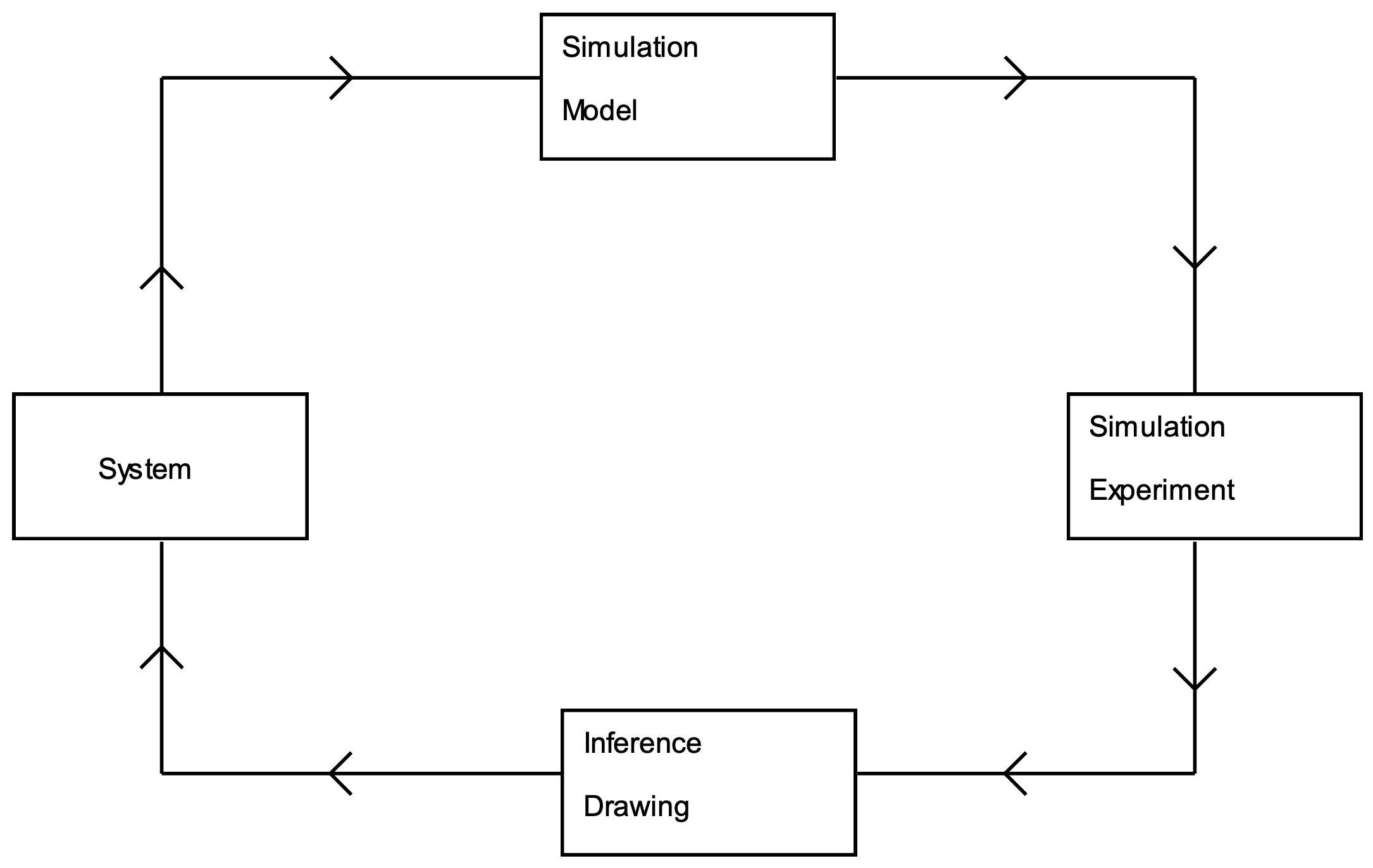
   A mathematical-logical form of an existing or proposed system, called a simulation model, is constructed (art). Experiments are conducted with the model that generates numerical results (science). The model and experimental results are interpreted to draw conclusions about the system (art). The conclusions are implemented in the system (science and art).

2. Simulation models emphasize the direct representation of the structure and logic of a system as opposed to abstracting the system into a strictly mathematical form. The availability of system descriptions and data influences the choice of simulation model parameters as well as which system objects and which of their attributes can be included in the model. Thus, simulation models are analytically intractable, that is exact values of quantities that measure system performance cannot be derived from the model by mathematical analysis. Instead, such inferencing is accomplished by experimental procedures that result in statistical estimates of values of interest. Simulation experiments must be designed as would any laboratory or field experiment. Proper statistical methods must be used in observing performance measure values and in interpreting experimental results.
3. Computer simulation models can be implemented and experiments conducted at a fraction of the cost of the P-D-C-A cycle of lean used to improve the future state to reach operational performance objectives. Simulation models are more flexible and adaptable to changing requirements than P-D-C-A. Alternatives can be assessed without the fear that negative consequences will damage day-to-day operations. Thus, a great variety of options can be considered at a small cost and with little risk.

   For example, suppose a lean team want to know if a new proposed layout for a manufacturing facility would increase the throughput and reduce the cycle time. The existing layout could be changed and the results measured, consistent with the lean approach. Alternatively, simulation could be used to assess the impact of the proposed new layout.

4. As was discussed in the previous section, simulation projects can result in the iterative definition of models and experimentation with models. Simulation languages and software environments are constructed to help models evolve as project requirements change and become more clearly defined over time.
5. A simulation model should be built to address a clearly specified set of system design and operation issues. These issues help distinguish the significant system objects and relationships to include in the model from those that are secondary and thus may be eliminated or approximated. This approach places bounds on what can be learned from the model. Care should be taken not to use the model to extrapolate beyond the bounds.
6. "Garbage in - garbage out" applies to models and their input parameter values (Sargent, 2009).

   A model must accurately represent a system and data used to estimate model input parameter values must by correctly collected and statistically analyzed. This is illustrated in Figure 1-3.

   Figure 1-3: Model Validation and Verification.

   

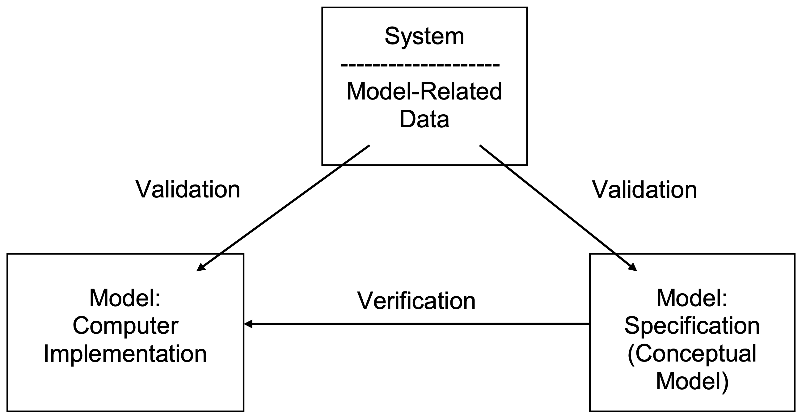
   There are two versions of a simulation model, the one specified "on paper" (the conceptual model) in the first strategic phase of the project process and the one implemented in the computer in the second strategic phase. Verification is the process of making sure these two are equivalent. Verification is aided, at least in part, by expressing the "on paper" model in a graphical drawing whose computer implementation is automatically performed.

   Validation involves compiling evidence that the model is an accurate representation of the system with respect to the solution objectives and thus results obtained from it can be used to make decisions about the system under study. Validation has to do with comparing the system and the data extracted from it to the two simulation models and experimental results. Conclusions drawn from invalid models could lead to system "improvements" that make system performance worse instead of better. This makes simulation and system designers who use it useless in the eyes of management.

7. A story is told of a young university professor who was teaching an industrial short course on simulation. He gave a lengthy and detailed explanation of a sophisticated technique for estimating the confidence interval of the mean. At the next break, a veteran engineer took him aside and said "I appreciate your explanation, but when I design a system I pretty much know what the mean is. It is the variation and extremes in system behavior that kill me."

   Variation has to do with the reality that no system does the same activity in exactly the same way or in the same amount of time always. Of course, estimating the mean system behavior is not unimportant. On the other hand, if every aspect of every system operation always worked exactly on the average, system design and improvement would be much easier tasks. One of the deficiencies of lean is that such an assumption is often implicitly made.

   Variation may be represented by the second central moment of a statistical distribution, the variance. For example, the times between arrivals to a fast food restaurant during the lunch hour could be exponentially distributed with mean 10 seconds and, therefore, variance 100 seconds. Variation may also arise from decision rules that change processing procedures based on what a system is currently doing or because of the characteristics of the unit being processed. For instance, the processing time on a machine could be 2 minutes for parts of type A and 3 minutes for parts of type B.

   There are two kinds of variation in a system: special effect and common cause. Special effect variation arises when something out of the ordinary happens, such as a machine breaks down or the raw material inventory becomes exhausted because of an unreliable supplier. Simulation models can show the step by step details of how a system responds to a particular special effect. This helps managers respond to such occurrences effectively.

   Common cause variation is inherent to a normally operating system. The time taken to perform operations, especially manual ones, is not always the same. Inputs may not be constantly available or arrive at equally spaced intervals in time. They may not all be identical and may require different processing based on particular characteristics. Scheduled maintenance, machine set up tasks, and worker breaks may all contribute. Often, one objective of a simulation study is to find and assess ways of reducing this variation.

   Common cause variation is further classified in three ways. Outer noise variation is due to external sources and factors beyond the control of the system. A typical example is variation in the time between customer orders for the product produced by the system. Variational noise is indigenous to the system such as the variation in the operation time for one process step. Inner noise variation results from the physical deterioration of system resources. Thus, maintenance and repair of equipment may be included in a model.

8. Computer-based simulation experiments result in multiple observations of performance measures. The variation in these observations reflects the common cause and special effect variation inherent in the system. This variation is seen in graphs showing all observations of the performance measures as well as histograms and bar charts organizing the observations into categories. Summary statistics, such as the minimum, maximum, and average, should be computed from the observations. Figure 1-4 shows three sample graphs.

   Figure 1-4: Example Graphs for Performance Measure Observations

   

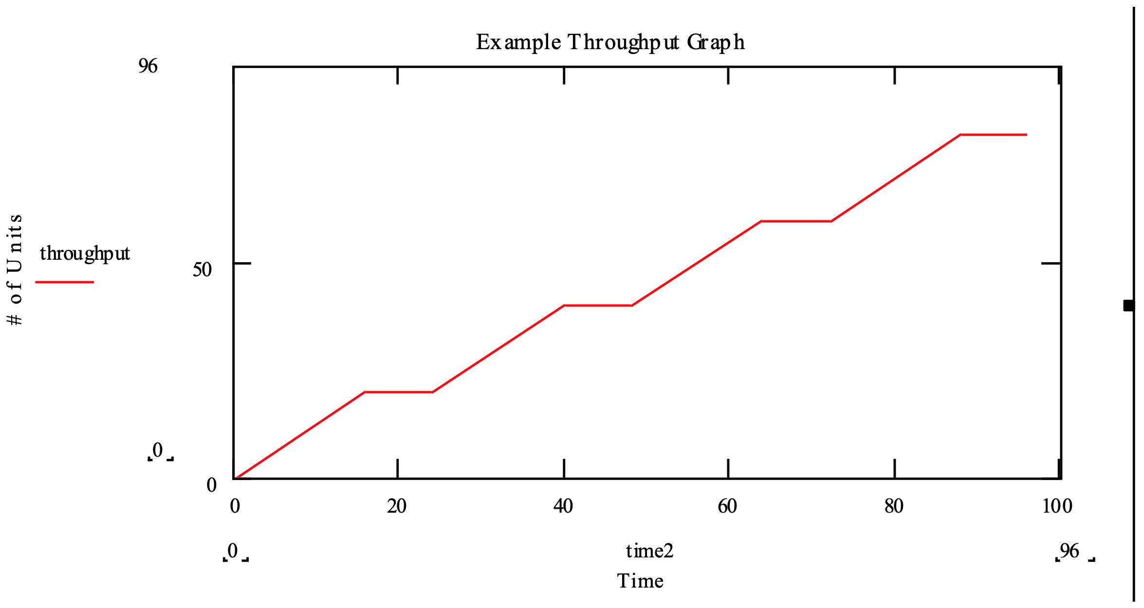
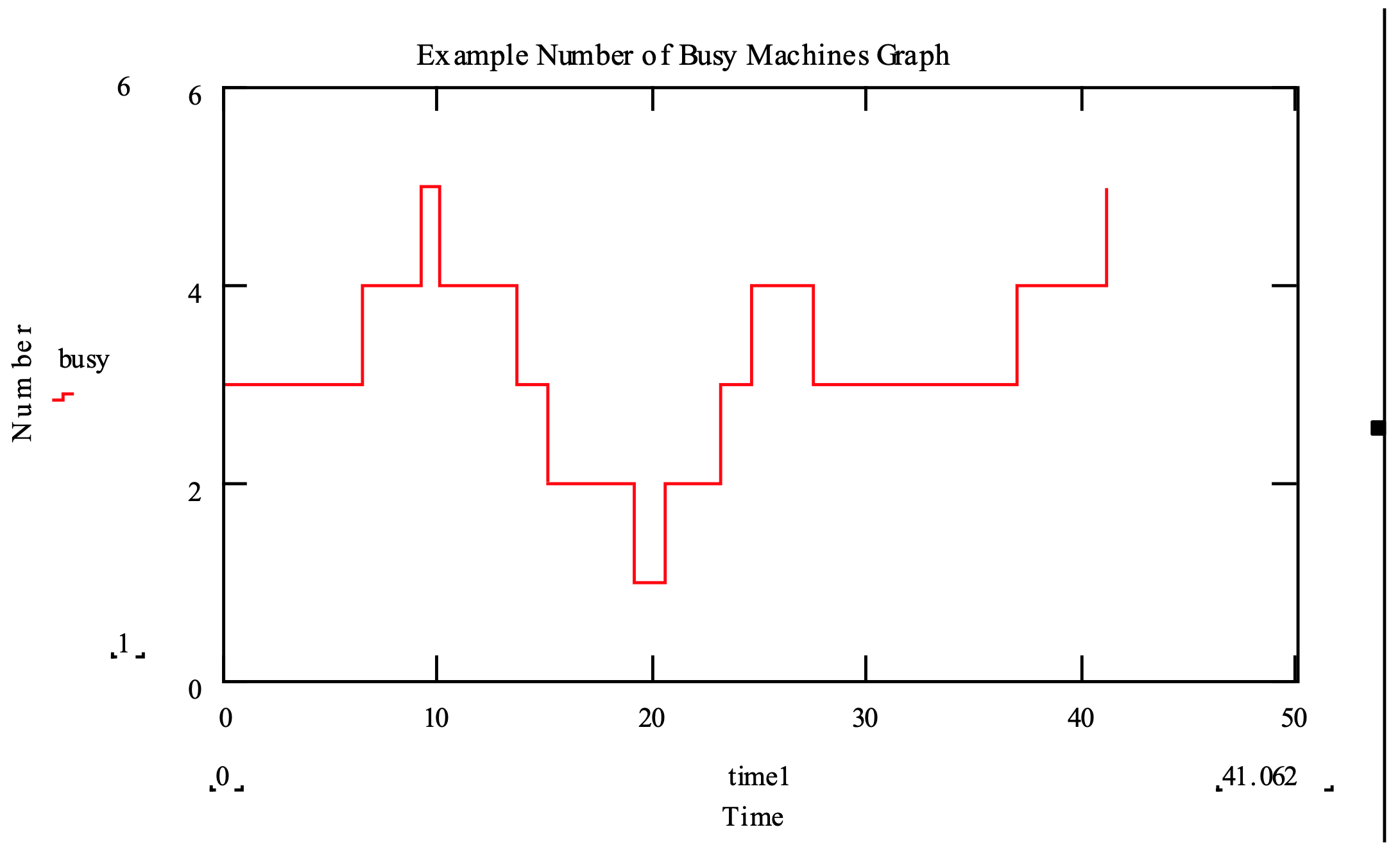
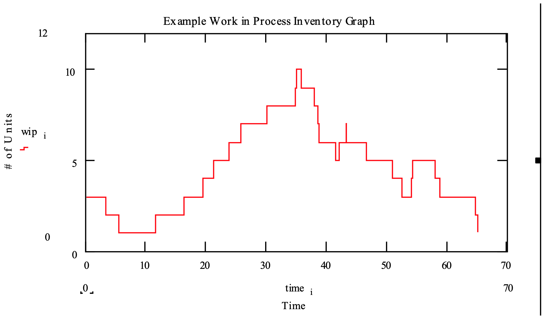
   The first shows how a special effect, machine failure, results in a build up of partially completed work. After the machine is repaired, the build up declines. The second shows the pattern of the number of busy machines at one system operation over time. The high variability suggests a high level of common cause variation and that work load leveling strategies could be employed to reduce the number of machines assigned to the particular task. The third graph shows the total system output, called throughput, over time. Note that there is no increase in output during shutdown periods, but otherwise the throughput rate appears to be constant.

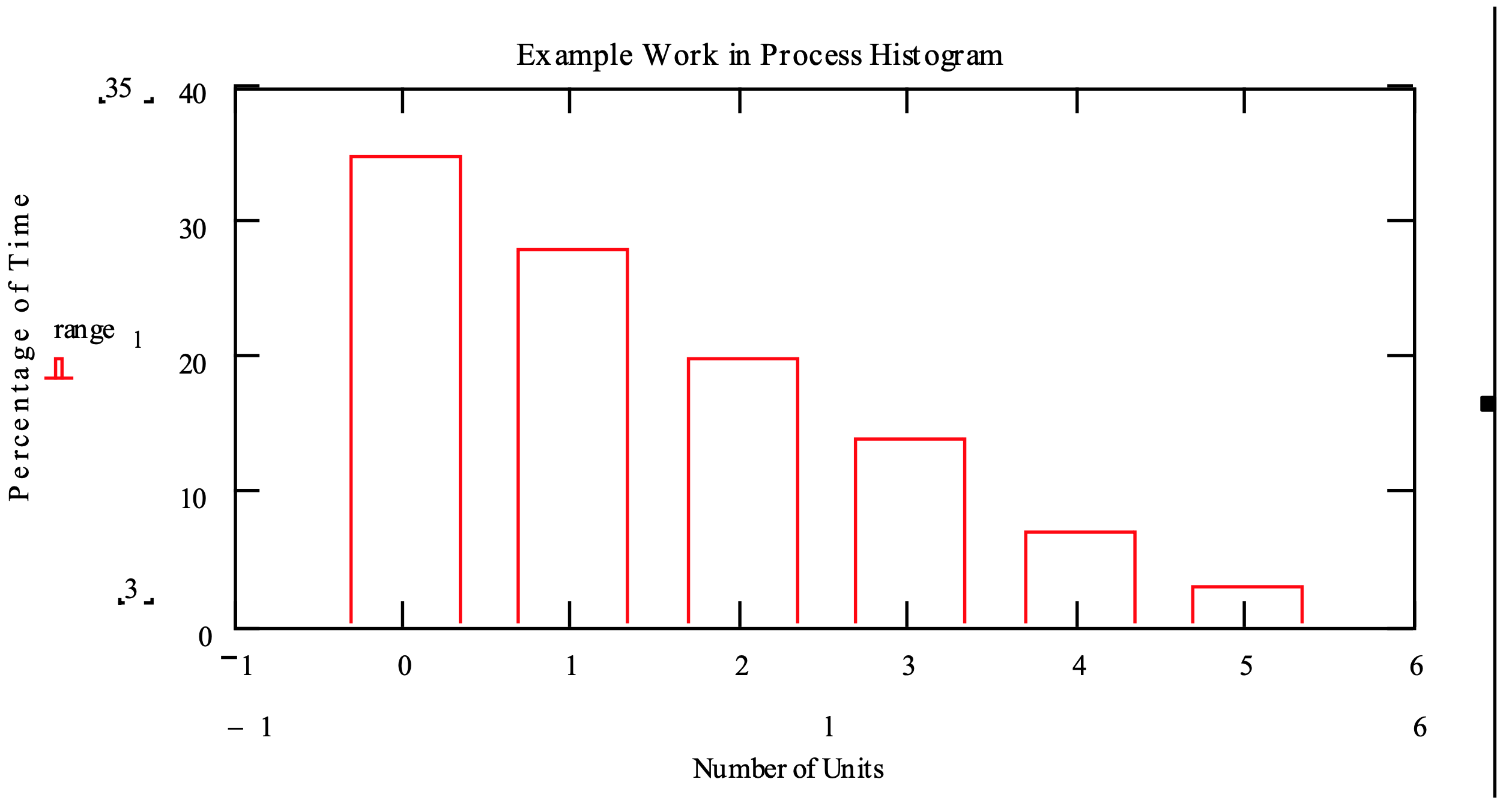
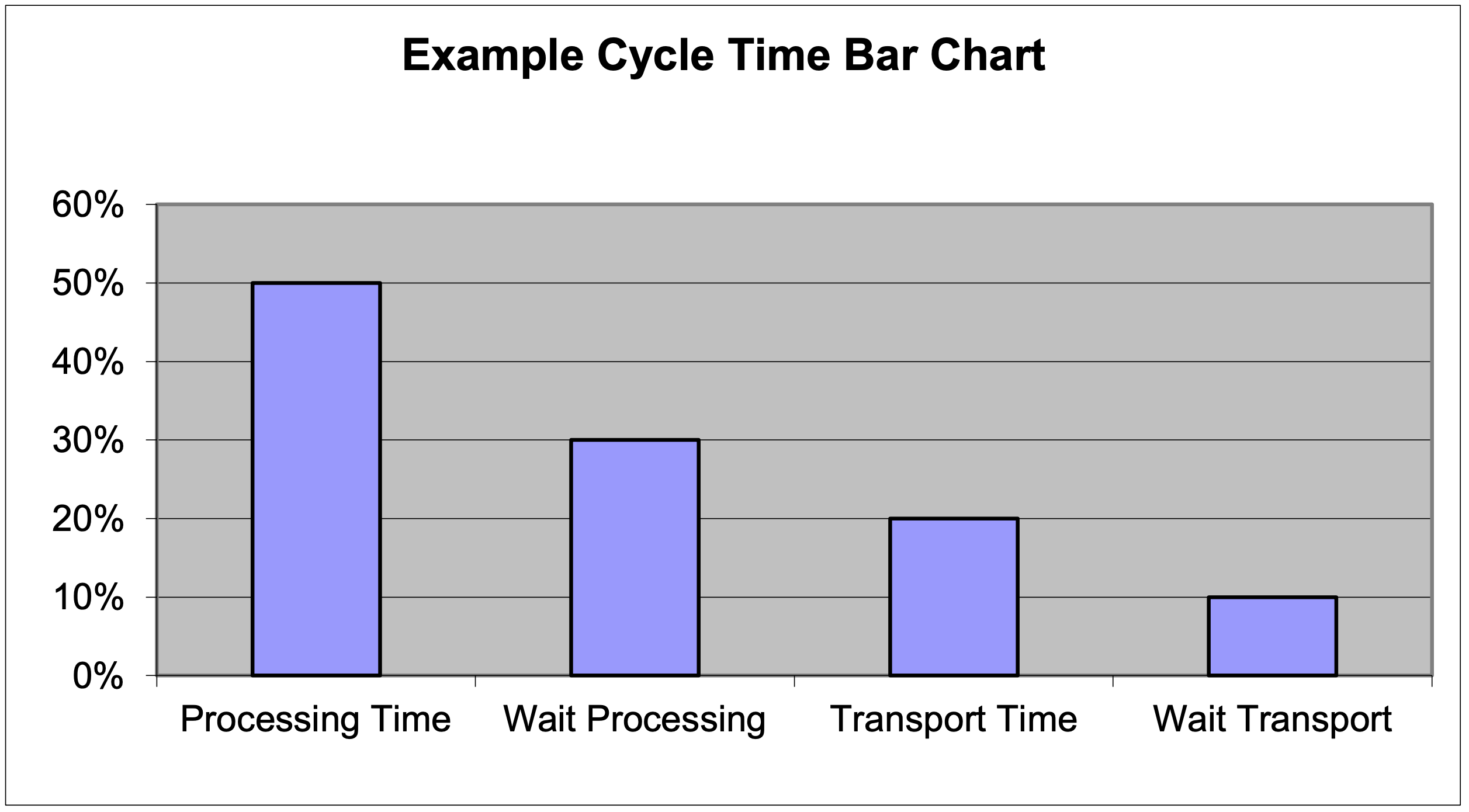
   Figure 1-5 shows a sample histogram and a sample bar chart. The histogram shows the sample distribution of the number of discrete parts in a system that appears to be acceptably low most of the time. The bar chart shows how these parts spend their time in the system. Note that one-half of the time was spent in actual processing which is good for most manufacturing systems.

   Figure 1-5: Example Histogram and Bar Charts for Performance Measure Observations

   

9. Using simulation, the analyst is free to define and compute any performance measure of interest, including those unique to a particular system. Transient or time varying behavior can be observed by examining individual observations of these quantities. Thus, simulation is uniquely able to generate information that leads to a thorough understanding of system design and operation.

   Though unique performance measures can be defined for each system, experience has shown that some categories of performance measures are commonly used:

   1. System outputs per time interval (throughput) or the time required to produce a certain amount of output (makespan).
   2. Waiting for system resources, both the number waiting and the waiting time.
   3. The amount of time, lead time, required to convert individual system inputs to system outputs.
   4. The utilization of system resources.
   5. Service level, the ability of the system to meet customer requirements.
10. Every unit entering a simulation model for processing should be accounted for either as exiting the model or assembled with other units or destroyed. Accounting for every unit aids in verification.
11. Analytic models can be used to enhance simulation modeling and experimentation. Result of analytic models can be used to set lower and upper bounds on system operating parameters such as inventory levels. Simulation experiments can be used to refine these estimates. Analytic models and simulation models can compute the same quantities, supporting validation efforts.
12. Simulation procedures are founded on the engineering viewpoint that solving the problem is of utmost importance. Simulation was born of the necessity to extract information from models where analytic methods could not. Simulation modeling, experimentation, and software environments have evolved since the 1950’s to meet expanding requirements for understanding complex systems.

    Simulation assists lean teams in building a consensus based on quantitative and objective information. This helps avoid “design by argument”. The simulation model becomes a valuable team member and is often the focus of team discussions.

    This principle is the summary of the rest. Problem solving requires that models conform to system structure and data (2) as well as adapting as project requirements change (4). Simulation enhances problem solving by minimizing the cost and risk of experimentation with systems (3). Information requirements for problem solving can be met (9). Analytic methods can be employed where helpful (11).