
2.3: Models of System Components
- Page ID
- 30962

\( \newcommand{\vecs}[1]{\overset { \scriptstyle \rightharpoonup} {\mathbf{#1}} } \)
\( \newcommand{\vecd}[1]{\overset{-\!-\!\rightharpoonup}{\vphantom{a}\smash {#1}}} \)
\( \newcommand{\dsum}{\displaystyle\sum\limits} \)
\( \newcommand{\dint}{\displaystyle\int\limits} \)
\( \newcommand{\dlim}{\displaystyle\lim\limits} \)
\( \newcommand{\id}{\mathrm{id}}\) \( \newcommand{\Span}{\mathrm{span}}\)
( \newcommand{\kernel}{\mathrm{null}\,}\) \( \newcommand{\range}{\mathrm{range}\,}\)
\( \newcommand{\RealPart}{\mathrm{Re}}\) \( \newcommand{\ImaginaryPart}{\mathrm{Im}}\)
\( \newcommand{\Argument}{\mathrm{Arg}}\) \( \newcommand{\norm}[1]{\| #1 \|}\)
\( \newcommand{\inner}[2]{\langle #1, #2 \rangle}\)
\( \newcommand{\Span}{\mathrm{span}}\)
\( \newcommand{\id}{\mathrm{id}}\)
\( \newcommand{\Span}{\mathrm{span}}\)
\( \newcommand{\kernel}{\mathrm{null}\,}\)
\( \newcommand{\range}{\mathrm{range}\,}\)
\( \newcommand{\RealPart}{\mathrm{Re}}\)
\( \newcommand{\ImaginaryPart}{\mathrm{Im}}\)
\( \newcommand{\Argument}{\mathrm{Arg}}\)
\( \newcommand{\norm}[1]{\| #1 \|}\)
\( \newcommand{\inner}[2]{\langle #1, #2 \rangle}\)
\( \newcommand{\Span}{\mathrm{span}}\) \( \newcommand{\AA}{\unicode[.8,0]{x212B}}\)
\( \newcommand{\vectorA}[1]{\vec{#1}} % arrow\)
\( \newcommand{\vectorAt}[1]{\vec{\text{#1}}} % arrow\)
\( \newcommand{\vectorB}[1]{\overset { \scriptstyle \rightharpoonup} {\mathbf{#1}} } \)
\( \newcommand{\vectorC}[1]{\textbf{#1}} \)
\( \newcommand{\vectorD}[1]{\overrightarrow{#1}} \)
\( \newcommand{\vectorDt}[1]{\overrightarrow{\text{#1}}} \)
\( \newcommand{\vectE}[1]{\overset{-\!-\!\rightharpoonup}{\vphantom{a}\smash{\mathbf {#1}}}} \)
\( \newcommand{\vecs}[1]{\overset { \scriptstyle \rightharpoonup} {\mathbf{#1}} } \)
\(\newcommand{\longvect}{\overrightarrow}\)
\( \newcommand{\vecd}[1]{\overset{-\!-\!\rightharpoonup}{\vphantom{a}\smash {#1}}} \)
\(\newcommand{\avec}{\mathbf a}\) \(\newcommand{\bvec}{\mathbf b}\) \(\newcommand{\cvec}{\mathbf c}\) \(\newcommand{\dvec}{\mathbf d}\) \(\newcommand{\dtil}{\widetilde{\mathbf d}}\) \(\newcommand{\evec}{\mathbf e}\) \(\newcommand{\fvec}{\mathbf f}\) \(\newcommand{\nvec}{\mathbf n}\) \(\newcommand{\pvec}{\mathbf p}\) \(\newcommand{\qvec}{\mathbf q}\) \(\newcommand{\svec}{\mathbf s}\) \(\newcommand{\tvec}{\mathbf t}\) \(\newcommand{\uvec}{\mathbf u}\) \(\newcommand{\vvec}{\mathbf v}\) \(\newcommand{\wvec}{\mathbf w}\) \(\newcommand{\xvec}{\mathbf x}\) \(\newcommand{\yvec}{\mathbf y}\) \(\newcommand{\zvec}{\mathbf z}\) \(\newcommand{\rvec}{\mathbf r}\) \(\newcommand{\mvec}{\mathbf m}\) \(\newcommand{\zerovec}{\mathbf 0}\) \(\newcommand{\onevec}{\mathbf 1}\) \(\newcommand{\real}{\mathbb R}\) \(\newcommand{\twovec}[2]{\left[\begin{array}{r}#1 \\ #2 \end{array}\right]}\) \(\newcommand{\ctwovec}[2]{\left[\begin{array}{c}#1 \\ #2 \end{array}\right]}\) \(\newcommand{\threevec}[3]{\left[\begin{array}{r}#1 \\ #2 \\ #3 \end{array}\right]}\) \(\newcommand{\cthreevec}[3]{\left[\begin{array}{c}#1 \\ #2 \\ #3 \end{array}\right]}\) \(\newcommand{\fourvec}[4]{\left[\begin{array}{r}#1 \\ #2 \\ #3 \\ #4 \end{array}\right]}\) \(\newcommand{\cfourvec}[4]{\left[\begin{array}{c}#1 \\ #2 \\ #3 \\ #4 \end{array}\right]}\) \(\newcommand{\fivevec}[5]{\left[\begin{array}{r}#1 \\ #2 \\ #3 \\ #4 \\ #5 \\ \end{array}\right]}\) \(\newcommand{\cfivevec}[5]{\left[\begin{array}{c}#1 \\ #2 \\ #3 \\ #4 \\ #5 \\ \end{array}\right]}\) \(\newcommand{\mattwo}[4]{\left[\begin{array}{rr}#1 \amp #2 \\ #3 \amp #4 \\ \end{array}\right]}\) \(\newcommand{\laspan}[1]{\text{Span}\{#1\}}\) \(\newcommand{\bcal}{\cal B}\) \(\newcommand{\ccal}{\cal C}\) \(\newcommand{\scal}{\cal S}\) \(\newcommand{\wcal}{\cal W}\) \(\newcommand{\ecal}{\cal E}\) \(\newcommand{\coords}[2]{\left\{#1\right\}_{#2}}\) \(\newcommand{\gray}[1]{\color{gray}{#1}}\) \(\newcommand{\lgray}[1]{\color{lightgray}{#1}}\) \(\newcommand{\rank}{\operatorname{rank}}\) \(\newcommand{\row}{\text{Row}}\) \(\newcommand{\col}{\text{Col}}\) \(\renewcommand{\row}{\text{Row}}\) \(\newcommand{\nul}{\text{Nul}}\) \(\newcommand{\var}{\text{Var}}\) \(\newcommand{\corr}{\text{corr}}\) \(\newcommand{\len}[1]{\left|#1\right|}\) \(\newcommand{\bbar}{\overline{\bvec}}\) \(\newcommand{\bhat}{\widehat{\bvec}}\) \(\newcommand{\bperp}{\bvec^\perp}\) \(\newcommand{\xhat}{\widehat{\xvec}}\) \(\newcommand{\vhat}{\widehat{\vvec}}\) \(\newcommand{\uhat}{\widehat{\uvec}}\) \(\newcommand{\what}{\widehat{\wvec}}\) \(\newcommand{\Sighat}{\widehat{\Sigma}}\) \(\newcommand{\lt}{<}\) \(\newcommand{\gt}{>}\) \(\newcommand{\amp}{&}\) \(\definecolor{fillinmathshade}{gray}{0.9}\)Typical system components include arrivals, operations, routing, batching, and inventories. Models of these components are presented in this section. The models may be used directly, modified, extended, and combined to support the construction of new models of entire systems.
2.3.1 Arrivals
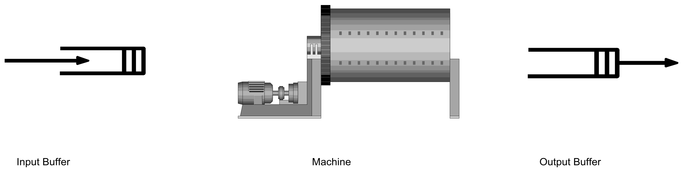
Consider a workstation with a single machine in a manufacturing facility as shown in Figure 2-1. One issue encountered when modeling the workstation is specifying at what simulated time each entity arrives. This specification includes the following:
- When the first entity arrives.
- The time between arrivals of entities, which could be a constant or a random variable modeled with a probability distribution. In a lean environment, the time between arrivals should equal the takt time as will be discussed in chapter 6.
- How many entities arrive during the simulation, which could be infinite or have an upper limit.
Suppose the first entity arrives at time 0, a common assumption in simulation modeling, and the time between arrivals is the same for all entities, a constant 10 seconds. Then the first arrival is at time 0, the second at time 10 seconds, the third at time 20 seconds, the fourth at time 30 seconds, and so forth.
Figure 2-1: Example Single Server (Machine) Workstation
Suppose that time between arrivals varies. This implies that the time between arrivals is describedbysomeprobabilitydistributionwhosemeanistheaveragetimebetweenarrivals. The variance of the distribution characterizes how much the individual times between arrivals differ from each other. For example, suppose the time between arrivals is exponentially distributed with mean 10 seconds, implying a variance of 10*10 = 100 seconds 2. The first arrival is at time 0. The second arrival could be at time 25 seconds, the third at time 31 seconds, the fourth at time 47 seconds, and so forth. Thus, the arrival process is a source of outer noise.
An example specification in pseudo-English follows.
| Define Arrivals: | // mean must equal takt time |
| \(\ \quad\quad\)Time of first arrival: | <>0 |
| \(\ \quad\quad\)Time between arrivals: | Exponentially distributed with a mean of 10 seconds Exponential (6) seconds |
| \(\ \quad\quad\)Number of arrivals: | Infinite |
2.3.2 Operations
The next issue encountered when modeling the single machine workstation in Figure 2-1 is specifying how the entities are processed by the workstation. Each entity must wait in the buffer (queue) preceding the machine. When available, the machine processes the entity. Then the entity departs the workstation.
A workstation resource is defined with the name WS to have 1 unit with states BUSY and IDLE using the notation WS/1: States(BUSY, IDLE). It is assumed that all units of a resource are initially IDLE. The operation of the machine is modeled as follows. Each entity waits for the single unit of the WS (workstation) resource to be available to operate on it that is the WS resource to be in the IDLE state. At the time processing begins WS becomes BUSY. After the operation time, the entity no longer needs WS, which becomes IDLE and available to operate on the next entity.
This may be expressed with the following statements:
| Define Resources: | WS/1 with states (Busy, Idle) |
| \(\ \quad\quad\)Process Single Workstation | |
| Begin | |
| \(\ \quad\quad\)Wait until WS/1 is Idle in Queue QWS | // part waits for its turn on the machine |
| \(\ \quad\quad\)Make WS/1 Busy | // part starts turn on machine; machine is busy |
| \(\ \quad\quad\)Wait for OperationTime | // part is processed |
| \(\ \quad\quad\)Make WS/1 Idle | // part is finished; machine is idle |
| End | |
Note the pattern of resource state changes. For every process step that makes a resource enter the busy state, there must be a corresponding step that makes the resource enter the idle state. However, there may be many process steps between these two corresponding steps. Thus, many operations may be performed in sequence on an entity using the same resource.
Note also the two types of wait statements that delay entity movement through a process. Wait for means wait for a specified amount of simulation time to pass. Wait unit means wait until a state variable value meets a specified logical condition. This is a very powerful construct that also is consistent with ideas in event-based programming.
Consider another variation on the single machine workstation operation that illustrates the use of conditional logic in a simulation model. The machine requires a setup operation of 1.5 minutes duration whenever the Type of an entity differs from the Type of the preceding entity processed by the machine. For example, the machine may require one set of operational parameter settings when operating on one type of part and a second set when operating on a second type of part. The model of this situation is as follows.
| Define Resources: \(\ \quad\quad\) WS/1 with states (Busy, Idle, Setup) |
|
| Define State Variables: \(\ \quad\quad\) LastType |
|
| Define Entity Attributes: \(\ \quad\quad\) Type |
|
| Process Single Workstation with Setup | |
| Begin | |
| \(\ \quad\quad\) Wait until WS/1 is Idle in Queue QWS | // part waits for its turn on the machine |
| \(\ \quad\quad\) Make WS/1 Busy | // part starts turn on machine; machine is busy |
| \(\ \quad\quad\) If LastType ! = Type then | |
| \(\ \quad\quad\) Begin | |
| \(\ \quad\quad\quad\quad\) Make WS/1 Setup \(\ \quad\quad\quad\quad\) Wait for SetupTime \(\ \quad\quad\quad\quad\) LastType = Type \(\ \quad\quad\quad\quad\) Make WS/1 Busy |
|
| \(\ \quad\quad\) End | |
| \(\ \quad\quad\) Wait for OperationTime | // part is processed |
| \(\ \quad\quad\) Make WS/1 Idle | // part is finished; machine is idle |
| End | |
A state variable, LastType stores the type of the last entity operated upon by the resource WS. Notice the use of conditional logic. Setup is performed depending on the sequence of entity types. Such logic is common in simulation models and makes most of them analytically intractable. A new state, SETUP, is defined for WS. This resource enters the SETUP state when the setup operation begins and returns to the BUSY state when the setup operation ends.
Often a workstation is subject to interruptions. In general, there are two types of interruptions: scheduled and unscheduled. Scheduled interruptions occur at predefined points in time. Scheduled maintenance, work breaks during a shift, and shift changes are examples of scheduled interruptions. The duration of a scheduled interruption is typically a constant amount of time. Unscheduled interruptions occur randomly. Breakdowns of equipment can be viewed as unscheduled interruptions. An unscheduled interruption typically has a random duration.
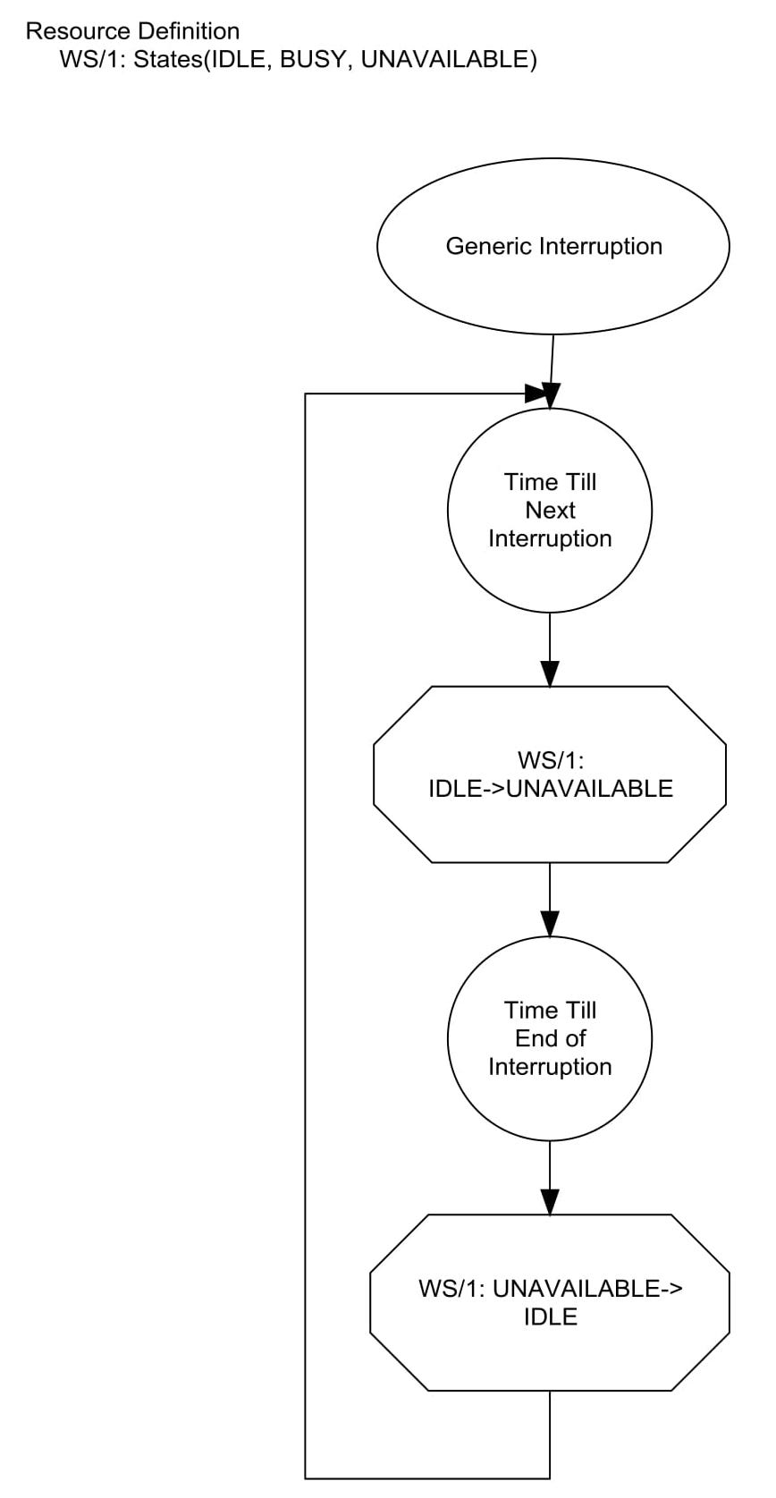
A generic model of interruptions is shown in Figure 2-2. An interruption occurs after a certain amount of operating time that is either constant or random. The duration of the interrupt is either constant or random. After the end of the interruption, this cycle repeats.
Note that the transition to the INTERRUPTED state is modeled as occurring from the IDLE state. Suppose the resource is in the BUSY state when the interruption occurs. Typically, a simulation engine will assume that the resource finishes a processing step before entering the INTERRUPTED state. However, the end time of the interruption will be the same that is the amount of time in the INTERRUPTED state will be reduced by the time spent after the interruption occurs in the BUSY state. This approximation normally has little or no effect on the simulation results. In many systems, interruptions are often only detected or acted upon at the end of an operation. Using this approximation avoids having to include logic in the model as to what to do with the entity being processed when the interruption occurs. On the other hand, such logic could be included in the model if required.
This breakdown-repair process may be expressed in statements as follows:
| Define Resource: \(\ \quad\quad\) WS/1: States(Busy, Idle, Unavailable) |
|
| Process Breakdown—Repair | |
| Begin | |
| \(\ \quad\quad\) Do While 1=1 | // Do forever |
| \(\ \quad\quad\quad\quad\)Wait for TimeBetweenBreakdowns | |
| \(\ \quad\quad\quad\quad\)Wait until WS/1 is Idle | |
| \(\ \quad\quad\quad\quad\)Make WS/1 Unavailable | |
| \(\ \quad\quad\quad\quad\)Wait for RepairTime | |
| \(\ \quad\quad\quad\quad\)Make WS/1 Idle | |
| \(\ \quad\quad\)End Do | |
| End | |
Consider an extension of the model of the single machine workstation with breakdowns (random interruptions) added. This model combines the process model for the single workstation with the process model for breakdown and repair. The WS resource now has three states: BUSY operating on an entity, IDLE waiting for an entity, and UNAVAILABLE during a breakdown. This illustrates how a model can consist of more than one process.
This model illustrates one of the most powerful capabilities of simulation. Two processes can change the state of the same resource but otherwise do not transfer information between each other. Thus, processes can be built in parallel and changed independently of each other as well as added to the model or deleted from the model as necessary. Thus, simulation models can be built, implemented, and evolved piece by piece.
Figure 2-2: Generic Interruption Process
2.3.3 Routing Entities
In many systems, decisions must be made about the routing of entities from operation to operation. This section discusses typical ways systems make such routing decisions as well as techniques for modeling them. A distinct process for making the routing decision can be included in the model.
Consider a system that processes multiple item types using several workstations. Each workstation performs a unique function. Each job type is operated on by a unique sequence of workstations called a route. In a manufacturing environment, this style of organization is referred to as a job shop. It could also represent the movement of customers through a cafeteria where different foods: hot meals, sandwiches, salads, desserts, and drinks are served at different stations. Customers are free to visit the stations in any desired sequence.
Each entity in the model of a job shop organization could have the following attributes:
| ArrivalTime: | Time of arrival |
| Type: | The type of job, which implies the route. |
| Location: | The current location on the route relative to the beginning of the route. |
In addition, the model needs to store the route for each type of job.
Suppose there are four workstations and three job types in a system. Figure 2-3 shows a possible set of routings in matrix form.
| Job Type | First Operation | Second Operation | Third Operation | Fourth Operation |
| 1 | Workstation 1 | Workstation 2 | Workstation 3 | Workstation 4 |
| 2 | Workstation 3 | Workstation 4 | None | None |
| 3 | Workstation 4 | Workstation 2 | Workstation 3 | None |
Figure 2-3: Example Routing Matrix for A Manufacturing Facility.
A routing process is included in the simulation model to direct the entity to the workstation performing the next processing step. The routing process requires zero simulation time.
Define State Variable:
\(\ \quad\quad\) Route(3, 4)
Define Attribute:
\(\ \quad\quad\) Location
Define Attribute:
\(\ \quad\quad\) Type
Process Routing
Begin
\(\ \quad\quad\)Location += 1
\(\ \quad\quad\)If Route(Type, Location) != None Then
\(\ \quad\quad\)Begin
\(\ \quad\quad\quad\quad\)Send to Process Route(Type, Location)
\(\ \quad\quad\)End
\(\ \quad\quad\)Else Begin
\(\ \quad\quad\quad\quad\)Send to Process Depart
\(\ \quad\quad\)End
End
The value of the Location attribute is incremented by one. The next workstation to process the entity is the one at matrix location (Type, Location). If this matrix location has a value of None, then processing of the entity is complete. Note again that the ability to compose a model of multiple processes is important.
Alternatively, routes may be selected dynamically based on current conditions in a system as captured in the values of the state variables. Such decision making may be included in a simulation model. This is another unique and very powerful capability of simulation modeling.
Consider a highly automated system in which parts wait in a central storage area for processing at any workstation. A robot moves the parts between the central storage area and the workstations. Alternatively if the following workstation is IDLE when an operation is completed, the robot moves the part directly to the next workstation instead of the storage area. The routing process for this situation follows, where WSNext is the resource modeling the following workstation.
Define Resource:
\(\ \quad\quad\) WSNext/1: States(Busy, Idle)
Define State Variable:
\(\ \quad\quad\) CentralStorage
Process Conditional Routing
Begin
\(\ \quad\quad\) If WSNext/1 is Idle Then
\(\ \quad\quad\) Begin
\(\ \quad\quad\quad\quad\) Send to Process ForWSnext
\(\ \quad\quad\) End
\(\ \quad\quad\) Else Begin
\(\ \quad\quad\quad\quad\) CentralStorage += 1
\(\ \quad\quad\)End
End
2.3.4 Batching
Many systems use a strategy of grouping items together and then processing all the items in the group jointly. This strategy is called batching. Batching may occur preceding a machine on the factory floor. Parts of the same type are grouped and processed together in order to avoid frequent setup operations. Other examples include:
- Bags of product may be stacked on a pallet until its capacity is reached. Then a forklift could be used to load the pallet on a truck for shipment.
- All deposits and checks received by a bank during the day are sent together to a processing center where bank account records are updated overnight.
- A tram operating from the parking lot in an amusement park to the entrance gate waits at the stop until a certain number of passengers have boarded.
Batching is the opposite of the lean concept of one-piece flow or one part per batch. There is a trade-off between batching and one-piece flow. Batching minimizes set up times and can make individual machines more productive. One-piece flow minimizes lead time, the time between starting production on a part and completing it, as well as in-process inventories.
Batching may be modeled by creating one group entity consisting of multiple individual entities. The group entity can be operated upon and routed as would an individual entity. Batching can be undone, that is the group can be broken up into the original individual entities.
Returning to the single server workstation example of Figure 2-2, suppose that completed parts are transported in groups of 20 from the output buffer to input buffer of a second workstation some distance away. At the second workstation, items are processed individually. In the simulation model of this situation, the first 19 entities, each modeling an item to be transported, must wait until the twentieth entity arrives. Then the 20 entities are moved together as a group. Each group is referred to as a batch. Upon arrival at the second workstation, each entity individually enters the workstation buffer. The batching and un-batching extension to the single server workstation model is as follows.
| Define Resource: | WS/1: States(Busy, Idle) |
| Define List: | OutputBuffer |
| Process Single Workstation with Output Buffer | |
|
Begin \(\ \quad\quad\quad\quad\) Wait until WS/1 is Idle
\(\ \quad\quad\quad\quad\) If Length (OutputBuffer) < 19 then \(\ \quad\quad\quad\quad\quad\quad\) Send All Entities on List(OutputBuffer) to Process WS2 \(\ \quad\quad\quad\quad\) End End |
|
Consider the case where each of the types of items processed by the workstation must be transported separately. In this situation, batching, transportation, and un-batching can be done as above except one batch is formed for each type of item.
2.3.5 Inventories
In many systems, items are produced and stored for subsequent use. A collection of such stored items is called an inventory, for example televisions waiting in a store for purchase or hamburgers under the hot lamp at a fast food restaurant. Customers desiring a particular item must wait until one is inventory.
Inventory processes have to do with adding items to an inventory and removing items from an inventory. The number of items in an inventory can be modeled using a state variable, for example INV_LEVEL. Placing an item in inventory is modeled by adding one to the state variable: INV_LEVEL += 1. Modeling the removal of an item from an inventory requires two steps:
- Wait for an item to be in the inventory: WAIT UNTIL INV_LEVEL > 0
- Subtract one from the number of items in the inventory: INV_LEVEL -= 1