4.2: Verification and Validation

This section discusses the verification and validation of simulation models. Verification and validation, first described in principle 6 of chapter 1, have to do with building a high level of confidence among the members of a project team that the model can fulfill is objectives. Verification and validation are an important part of the simulation process particularly with respect to increasing model credibility among managers and system experts.

Verification has to do with developing confidence that the computer implementation of a model is in agreement with the conceptual model as discussed in chapter 1. In other works, the computer implementation of the model agrees with the specifications given in the conceptual model. Verification includes debugging the computer implementation of the model.

Validation has to do with developing confidence that the conceptual model and the implemented model represent the actual system with sufficient accuracy to support making decision about project issues and to meet the solution objectives. In other works, the computer implementation of the model and the conceptual model faithfully represent the actual system.

As described by many authors (Balci, 1994; Balci, 1996; Banks, Carson, Nelson, and Nicol, 2009; Carson, 2002; Law, 2007; Sargent, 2009), verification and validation require gathering evidence that the model and its computer implementation accurately represent the system under study with respect to project issues and solution objectives. Verification and validation are a matter of degree. As more evidence is obtained, the greater the degree of confidence that the model is verified and valid increases. It should be remember however that absolute confidence (100%) cannot be achieved. There will always be some doubt as to whether a model is verified and validated.

How to obtain verification and validation evidence and what evidence to obtain is case specific and requires knowledge of the problem and solution objectives. Some generally applicable strategies are discussed and illustrated in the following sections. The application studies, starting in chapter 6, provide additional examples. Application problems in the same chapters give students the opportunity to practice verification and validation.

Verification and validation strategies are presented separately for clarity of discussion. However in practice, verification and validation tasks often are intermixed with little effort to distinguish verification from validation. The focus of both verification and validation is on building confidence that the model can be used to meet the objectives of the project.

A pre-requisite to a proper simulation experiment is verifying and validating the model.

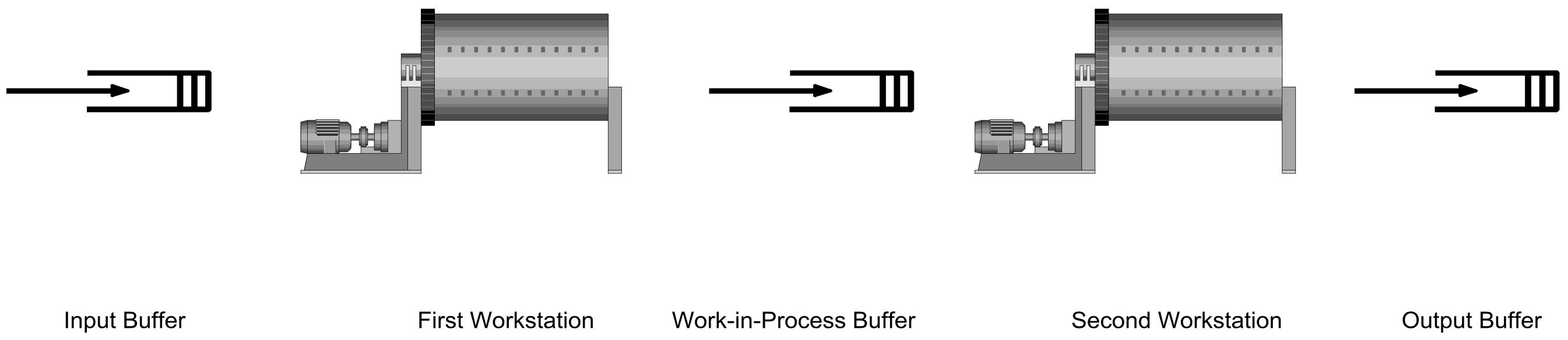
Throughout this chapter, including the discussion of verification and validation, illustrations and examples will make use of a model of two stations in a series with a large buffer between the stations as well as the industrial example presented in section 1.2. A diagram of the former is shown in Figure 4-1. A part enters the system, waits in the buffer of workstation A until the machine at this workstation is available. After processing at workstation A, a part moves to workstation B where it waits in the buffer until the workstation B machine is available. After processing at workstation B, a part leaves the system. Note that because it is large, the buffer between the stations is not modeled.

Figure 4-1: Example Two Workstations in Sequence, Repeated

4.2.1 Verification Procedures

Some generally applicable techniques for looking for verification evidence follow.

1. For example, in the two workstations in a series model, the following “entity balance” equation should hold:

   Number of entities entering the system =

   the number of entities departing the system + the number of entities still in the system at the end of the simulation

   The latter quantity consists of the number of entities in each workstation buffer (A and B) plus the number of entities being processed at workstations A and B. If the entity balance equality is not true, there is likely an error in the model that should be found and corrected.

   The number of entities entering the system consists of the number of entities initially there at the beginning of the simulation plus the number of entities arriving during the simulation.

   For example, for one simulation of the two workstations in a series model, there were 14359 entities arriving to the model of which 6 were there initially. There were 14357 entities that departed and two entities in the system at the end of the simulation. One of the two entities was in the workstation A operation and the other was in the workstation B operation.

2. The process steps in the model implemented in the computer version of the model and the conceptual model should correspond and any differences should be corrected or justified.

   The process steps in the two workstations in a series model are as follows:

   1. Arrive to the system.
   2. Enter the input buffer of workstation A.
   3. Be transformed by the workstation A operation.
   4. Be moved to and enter the input buffer of workstation B.
   5. Be transformed by the workstation B operation.
   6. Depart the system.
3. The model implementation should include the checking required to assure that input parameter values are correctly input and used.

   For example in the industrial application discussed in section 1.2, customer demand volume is input. The volume of product shipped is output. Enough information is included in the reports generated by the model to easily determine if all of the input volume is shipped or is awaiting shipment at the end of the simulation.

4. The time between arrivals is specified as part of the model. The average number of arrivals can be computed given the ending time of the simulation. In addition, the number of arrivals during the simulation run is usually automatically reported. These two quantities can be compared to assure that entities are being created as was intended.

   For example, suppose model of the two stations in a series was simulated for 40 hours with an average time between arrivals of 10 seconds. The expected number of arrivals would be 14400 (= 40 hours / 10 seconds). Suppose 20 independent simulations were made and the number of arrivals ranged from 14128 to 14722. Since this range includes 14400, verification evidence would be obtained. How to do the independent simulations is discussed in section 4.3 and following.

   Alternatively a confidence interval for the true mean number of arrivals could be computed. If this confidence interval includes the expected number of arrivals verification evidence is obtained. In the same example, the 95% confidence interval for the mean number of arrivals is 14319 to 14457. Again, verification evidence is obtained.

5. Sufficient checking should be built into the simulation model to assure that all logical decisions are correctly made that is all conditional logic is correctly implemented.

   For example in the industrial problem discussed in section 1.2, each product could be shipped from one of a specified set of loads spots. Output reports showed the volume of shipments by product and load spot combination. Thus, it could be easily seen if a product was shipped from the wrong load spot.

6. Verifying that any complex computer program was implemented as intended can be difficult. Implementing the smallest possible model helps simplify the verification task, and perhaps more importantly, results in a running model in relatively little time. Verifying one capability added to an already verified model is relatively straightforward.

   For example, the model of the industrial problem presented in section 1.2, has been developed over a number of years with new capabilities added to support addressing new issues and solution objectives.

7. Each individual implements an assigned portion of the model, or sub-model. Each individual presents the implementation to all of the other team members. The team as a whole must agree that the implementation faithfully represents the conceptual model.

   For example, one strategy is to build and implement an initial model as quickly as possible from the specifications in the conceptual model. If the conceptual model is incomplete, assumptions are made to complete model construction and implementation. The assumptions may be gross or inaccurate. The entire team reviews the initial model, especially the assumptions, and compares it to the conceptual model. The assumptions are corrected as necessary. This may require team members to gather additional information about how certain aspects of the system under study work.

8. Model builders implement the standard modeling constructs available in a simulation language. They provide a standard structure for model building and help guard against model building errors such as inconsistent or incomplete specification of modeling constructs.
9. Sufficient information should be output from the simulation to verify that the different components of the system are operating consistently with each other in the model.

   For example in the industrial problem of section 1.2, both the utilization of each load spot and summary statistics concerning the time to load each product are reported. If the load spots assigned to a product have high utilization, the average product loading time should be relatively long.

10. A model implementation can be verified only with respect to the particular set of model parameter values tested. Each new set of parameter values requires re-verification. However after many sets of parameter values have been tested, confidence is gained that the implementation is correct for all sets of parameter values in the same range.

    For example for the industrial problem of section 1.2, verification information is carefully examined after each simulation experiment.

4.2.2 Validation Procedures

Some generally applicable techniques for looking for validation evidence follow.

1. This is a restatement of principle 11 of chapter 1. For example, the mean number of busy units of a resource can be computed easily as discussed in chapter 6.

   In the two workstations in a series model, suppose the operation time at the second workstation is a constant 8.5 seconds and the mean time between arrivals is 10 seconds. The percentage busy time for workstation B is equal to 8.5 / 10 seconds or 85%. The simulation of the workstation provides data from which to estimate the percent busy time. The range of workstation B utilization over multiple independent simulations is 83% to 87%. A confidence interval for the true mean utilization could be computed as well. The 95% confidence interval is 84.4 to 85.4. Thus, validation evidence is obtained.

2. Reviewing all the implications of complex decisions using voluminous information in a static medium, such as a report, or even in an interactive debugger, is difficult and possibly overwhelming. Animation serves to condense and simplify the viewing of such information.

   Consider the following illustration. In the early 1980’s, a particular simulation company was developing its first commercial animator product. Having completed the implementation and testing, the development team asked an application consultant for an industrial model to animate. The consultant supplied a model that included a complex control system for a robot.

   The developers completed the animation and presented it to the consultant. The response of the consultant was that there must be something wrong with the new animation software as the robot could not engage in the sequence of behavior displayed.

   Try as they might, the development team could not find any software error in the animator. To aid them, the team asked the consultant to simulate the model, printing out all of the information about the robot’s behavior. The error was found not in the animator, but in the model. The disallowed behavior pattern occurred in the simulation!

   This is not a criticism of the consultant. Rather it points out how easy it was to see invalid behavior in an animation though it was infeasible to detect it through a careful examination of the model and output information.

3. System experts should review the model, parameter values and simulation results for consistency with system designs and expectations. Reports of simulation results should be presented in a format that is understandable to system experts without further explanation from the modelers. Animation can help in answering questions such as: How was the system represented in the model? Inconsistencies and unmet expectations must be resolved as either evidence of an invalid model or unexpected, but valid, system behavior.

   For example the development process for the industrial model discussed in section 1.2 was as follows. A first cut model was developed as quickly after the start of the project as possible. It was clear during the development of this model that some components of the system had not been identified or had incomplete specifications that is the first draft conceptual model was incomplete. The modelers made gross assumptions about how these components operated. The first cut model was reviewed by the entire project team including system experts and managers. Based on this review, tasks for completing the conceptual model were assigned. When these tasked were completed, the conceptual model was updated and the implemented model was revised accordingly.

4. As discussed in chapter 3, there may be a lack of data available for estimating time delays or other quantities needed in a model. This is common when the simulation model is being used to assist in the design of a new system. For such quantities, it is essential to perform a sensitivity analysis. This involves running the model with a variety of values of each estimated quantity and observing the effect on performance measures. Estimated quantities that greatly effect system performance should be identified. Further study may be necessary to obtain a more precise estimate of their value.

   For example, there was little data concerning shipping times, the time between when a product left the plant and when it arrived at a customer, for the industrial model discussed in section 1.2. These times were believed to be directly related to some of the key performance measures estimated by the model. Thus, it was thought to be wise to refine them over time. Initially, shipping times were specified as triangularly distributed with estimates of the minimum, maximum, and modal times for all products in general supplied by logistics experts. Later additional data was available so that shipment times were available for each group of products. Still later, an analysis of data in the corporate information system was done to provide product specific shipping times. The simulation model was modified to allow any of the three shipping time options to be used for any product.

5. A model specific report of the step-by-step actions taken during a run can be generated by the simulation in a format that can be read by system experts and managers. A careful examination of such a report, though tedious, can help assure that the process steps included in the simulation model are complete and correctly interact with each other.

   For example, the sponsors of an industrial inventory management simulation required such a trace to assure that the model correctly captured the response of the actual system to certain disturbances. The trace was carefully examined by the sponsors and other system experts to gain confidence that the model was valid.

6. The same performance measures computed in the model may be estimated from data collected from an existing system. Summary statistics, such as the average, computed from performance measure values may be compared by inspection to summary statistics computed from the data collected from an existing system. If no operationally significant differences are observed, then validation evidence is obtained.

   Law (2007) discusses the difficulty of using statistical tests to compare performance measure values and real world data as well as making some recommendations in this regard.

   For example, in the industrial model of section 1.2, system experts believed that empty rail cars spent 6 to 7 days in the plant. Simulation results estimated that empty rail cars spent an average of 6.6 days in the plant. Thus, validation evidence was obtained.