5.6: Random Sampling from Distribution Functions

Last updated
Save as PDF

Page ID: 30980

\( \newcommand{\vecs}[1]{\overset { \scriptstyle \rightharpoonup} {\mathbf{#1}} } \) \( \newcommand{\vecd}[1]{\overset{-\!-\!\rightharpoonup}{\vphantom{a}\smash {#1}}} \)\(\newcommand{\id}{\mathrm{id}}\) \( \newcommand{\Span}{\mathrm{span}}\) \( \newcommand{\kernel}{\mathrm{null}\,}\) \( \newcommand{\range}{\mathrm{range}\,}\) \( \newcommand{\RealPart}{\mathrm{Re}}\) \( \newcommand{\ImaginaryPart}{\mathrm{Im}}\) \( \newcommand{\Argument}{\mathrm{Arg}}\) \( \newcommand{\norm}[1]{\| #1 \|}\) \( \newcommand{\inner}[2]{\langle #1, #2 \rangle}\) \( \newcommand{\Span}{\mathrm{span}}\) \(\newcommand{\id}{\mathrm{id}}\) \( \newcommand{\Span}{\mathrm{span}}\) \( \newcommand{\kernel}{\mathrm{null}\,}\) \( \newcommand{\range}{\mathrm{range}\,}\) \( \newcommand{\RealPart}{\mathrm{Re}}\) \( \newcommand{\ImaginaryPart}{\mathrm{Im}}\) \( \newcommand{\Argument}{\mathrm{Arg}}\) \( \newcommand{\norm}[1]{\| #1 \|}\) \( \newcommand{\inner}[2]{\langle #1, #2 \rangle}\) \( \newcommand{\Span}{\mathrm{span}}\)\(\newcommand{\AA}{\unicode[.8,0]{x212B}}\)

In chapter 2, entity attribute values and the time between entity arrivals as well as operation and transportation times were modeled using probability distributions. Furthermore, values for these variables need to be assigned to each entity. To accomplish this assignment, a random sample must be taken from the corresponding probability distribution. This subject is worthy of a lengthy and thorough discussion such as that provided in Law (2007) as well as Carson, Banks, Nelson, and Nicol (2009). Here one approach for taking random samples is presented to illustrate how this issue is addressed.

Consider the time between entity arrivals in the two workstations in a series model: exponential (10) seconds, where 10 is the average time between arrivals, TBA. This quantity follows the cumulative distribution function:

\(\ y=F(x)=1-e^{-x / T B A}=1-e^{-x / 10}\)

and therefore

\begin{align}x=-T B A \ln (1-y)=-10 \ln (1-y)\tag{5-1}\end{align}

In the same way, the service time at workstation A is uniformly distributed between a minimum and a maximum value (5 and 13 seconds) and therefore follows the cumulative distribution function:

\(\ \mathrm{y}=\mathrm{F}(\mathrm{x})=(\mathrm{x} \text { -minimum) } /(\text { maximum }-\text { minimum })=(\mathrm{x}-5) /(13-5)\)

and therefore

\(\ \begin{align}x=y^{*}(\text { maximum - minimum })+\text { minimum }=y^{*}(13-5)+5\tag{5-1}\end{align}\)

Notice that taking the inverse of the cumulative distribution reduces each case to the same problem, determining the value of y. Thus, this approach for taking a random sample is called the inverse-transformation method.

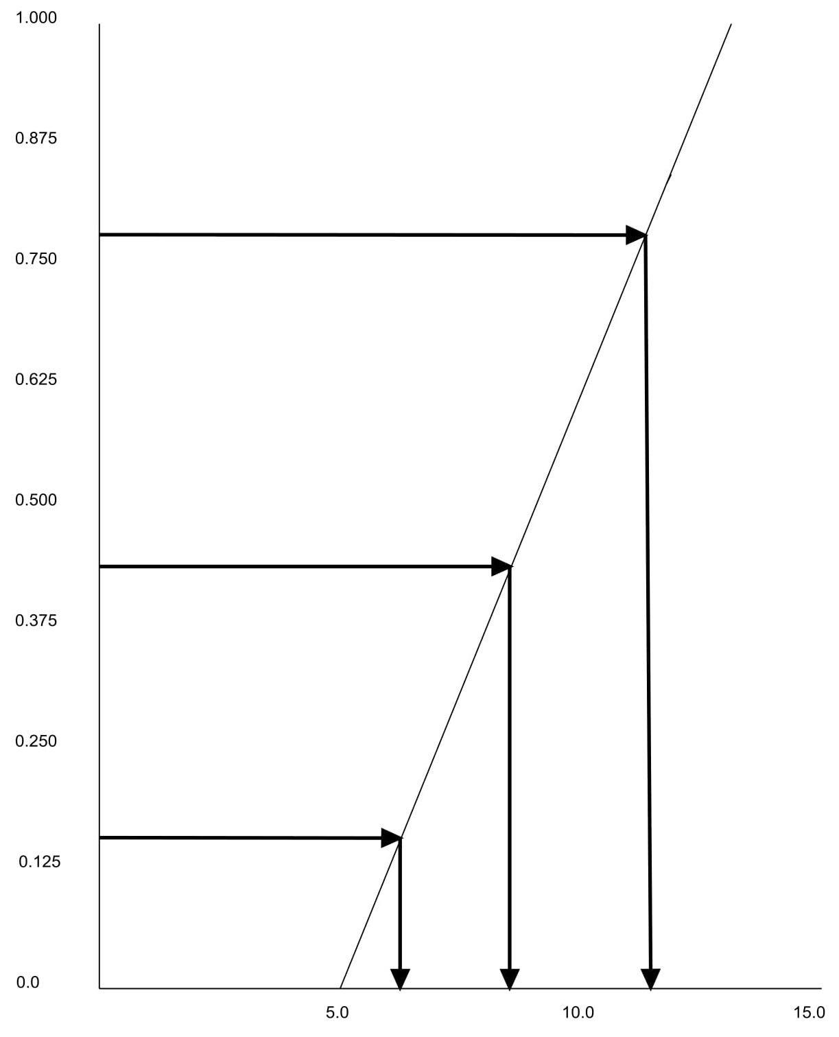
Figure 5-2 shows how this method works for the service time at workstation A. Any value of y in the range 0-1 is equally likely. (This is because y is a cumulative distribution.) Good experimental procedure requires a random sample and so a random sample of y must be chosen. Once a random value is selected for y, the random sample of x is straightforward to compute.

Work - Beyond Lean_ Simulation in Practice Second Edition-092.jpg

The inverse-transformation method is summarized as follows:

Determine the inverse of the cumulative distribution function, F^-1(x).
Each time a sample is needed:
1. Generate a random sample, r, uniformly distributed in the range 0 to 1.
2. x = F^-1(r).

Using the inverse-transformation method requires that the inverse of the cumulative distribution function exists. This is true for the following distributions commonly used in simulation models: uniform, triangular, exponential, weibull, and any discrete distribution where the mass function is enumerated as well as a heuristic distribution in histogram form.

As an example, consider the use of the inverse-transformation method with equation 5-2. Suppose r is selected to be 0.45. Then x = -10 ln (1 – 0.43) = 5.62. Next the inverse- transformation method is applied to equation 5-5. Suppose r is selected to be 0.88. Then x = 0.88 * ( 13 - 5 ) + 5 = 12.04.