6.3: The Case Study

The case study shows the process of using simulation and analytic models together to address issues concerning a new workstation before acquisition and implementation.

6.3.1 Define the Issues and Solution Objective

A lean team has been studying the operation of a particular workstation. A replacement machine with less variation in processing time, but the same average processing time, has been proposed as a part of a future state definition. Management is requiring a study to determine the average and maximum lead times at the workstation if the replacement machine is acquired.

The workstation operates 168 hours per month. Customer demand per month is 1680 parts or 10 parts per hour, resulting in a takt time of 6 minutes. The processing time for the new machine is triangularly distributed with a mean of 5 minutes, a minimum of 3 minutes and a maximum of 8 minutes. Thus, the mode is 4 minutes. (See the discussion in chapter 3 for the computation of the mode.) Inbound arrival of parts is not well controlled, which will be modeled using the practical worst case: Exponentially distributed with a mean equal to the takt time of 6 minutes.

6.3.2 Build Models

The model in pseudo-English is shown below.

---

Define Arrivals: \(\ \quad\quad\) Time of first arrival: \(\ \quad\quad\) Time between arrivals: \(\ \quad\quad\) Number of arrivals:	// mean must equal takt time 0 Exponentially distributed with a mean of 6 minutes Exponential (6) minutes Infinite // Note: The average number of arrivals is 1680
Define Resources: \(\ \quad\quad\) WS/1 with states (Busy, Idle)
Define Entity Attributes: \(\ \quad\quad\) ArrivalTime	// part tagged with its arrival time; each part has its own tag
Process Workstation
Begin \(\ \quad\quad\) Set ArrivalTime = Clock \(\ \quad\quad\) Wait until WS/1 is Idle in Queue QWS \(\ \quad\quad\) Make WS/1 Busy \(\ \quad\quad\) Wait for Triangular (3, 4, 8) minutes \(\ \quad\quad\) Make WS/1 Idle \(\ \quad\quad\) Tabulate (Clock-ArrivalTime) in LeadTime End	// record time part arrives on tag // part waits for its turn on the machine // part starts turn on machine; machine is busy // part is processed // part is finished; machine is idle // keep track of part time on machine

---

The definitions tell about arrivals, the machine including its states, and the entity (part) attributes. The comments (denoted by //) describe the steps the part goes through for processing on the machine as well as recording the arrival time and tabulating its individual lead time just before departure.

6.3.3 Identify Root Causes and Assess Initial Alternatives

In this section, the simulation experimental design and results are presented. First, an analytic model of the single work station is discussed in the next section.

6.3.3.1 Analytic Model of a Single Workstation

The time between arrivals is characterized by both a mean, T_a, and by a standard deviation, \(\ \sigma_a\) and the processing time is characterized by both its mean CT and by its standard deviation, \(\ \sigma_T\). The coefficient of variation of the time between arrivals is \(\ \mathrm{c}_{\mathrm{a}}=\sigma_{\mathrm{a}} / \mathrm{T}_{\mathrm{a}}\). The coefficient of variation of the processing time is \(\ \mathrm{c}_{\mathrm{T}}=\sigma_{\mathrm{T}} / \mathrm{C} \mathrm{T}\).

The average number of parts in the buffer is WIP_q and WIP_q plus the utilization of the machine (equal the average number of parts in processing) is the WIP.

The average time spent at the workstation can be broken into two parts: the average time in processing, CT, and the average time in the buffer, CT_q. Their sum is the total is the lead time LT.

The relationship between WIP, lead time and throughput is known as Little’s Law.

\(\ \begin{align}Work in process (WIP) = Throughput (TH) X Lead Time (LT)\tag{6-1}\end{align}\)

Examples:

Number of parts at a workstation =	Parts completed per hour at the work station X Total time at the workstation
Number of customers at Burger King =	Customers served per hour at Burger King X Time from entry to completion of service at BK
Number of pallets on a holding conveyor =	Pallets entering the main line conveyor per hour X Time till entry to the holding conveyor to entry to the main line conveyor
Number of units in a transfer center =	Number of units entering the transfer center per hour X Average processing time in the transfer center
Number of students enrolled at GVSU =	Number of students entering per year X Average number of years enrolled at GVSU

1. In order for the WIP (a bad thing to have lots of) to decrease, either the throughput must decrease (for a constant lead time) or the cycle time must decrease for a constant throughput. Since throughput often depends on requirements for finished goods and is the reciprocal of the takt time, decreasing lead time is most likely necessary to decrease WIP.
2. Another way of writing Little’s Law is TH = WIP / LT. This means that increasing throughput can be achieved by increasing WIP or decreasing LT. However, increasing WIP (a bad thing to have lots of) may increase lead time. Thus, increasing throughput most often requires decreasing lead time. Note that the same throughput can be achieved with large WIP and large lead times or small WIP and small lead times.
3. A third way of writing Little’s Law is LT = WIP / TH. Decreasing LT can be achieved by decreasing WIP or increasing throughput if the WIP does not increase.

Next we will consider all of the information that can be computed about the behavior of a single workstation that has one machine or one worker. We will include means and variances in evaluating average behavior. Notice that variation in measures of behavior is not, an often cannot, be determined analytically.

Consider the workstation shown in Figure 6-1, with computed quantities shown in boldface. Quantities that are known are the time between arrivals (mean and variance) as well as the processing time (mean and variance). Quantities that can be computed are:

1. time in the input buffer of the station (CT_q)
2. lead time at the station (LT)
3. average number of parts in the input buffer (WIP_q)
4. average number of parts at the station (WIP)
5. utilization of the station, the percent of time the workstation is busy processing a part. \(\ (\mu)\)
6. time between departures (mean and standard deviation) (T_d and \(\ \sigma\)_d)

Figure 6-1: Computation of Workstation Quantities

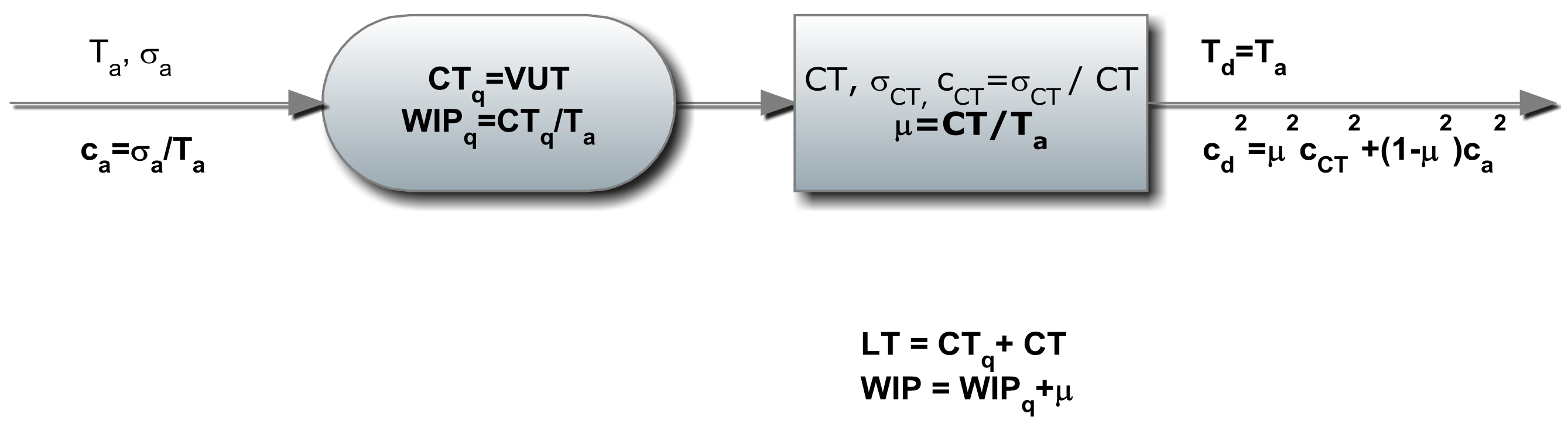
Equation 6-2 is called the VUT equation, for Variance – Utilization – Time and is used to approximate the average cycle time in the queue. This equation is presented and further discussed in Hopp and Spearman (2007).

\begin{align}C T_{q} \approx V U T=\left(\frac{c_{a}^{2}+c_{C T}^{2}}{2}\right)\left(\frac{\mu}{1-\mu}\right) C T\tag{6-2}\end{align}

The following insights can be gained by examining equation 6-2.

1. The cycle time in the buffer depends on the variance of the time between arrivals and the variance of the processing time, expressed as the squared coefficient of variation. As the variance of either increase, the average cycle time in the queue increases. The coefficient of variation is the standard deviation / mean.
2. The cycle time in the buffer increases in a highly non-linear fashion as the utilization increases. The utilization term for a utilization of 90% is 9, for a utilization of 95% is 19, and for a utilization of 99% is 99.
3. The only way to effectively run a workstation with high utilization is to eliminate the variation in the time between arrivals and the processing time.
4. A utilization of 100% cannot be achieved unless the variance in both the processing time and the time between arrivals is zero.
5. The mean and the standard deviation of the exponential distribution are equal. Thus, the coefficient of variation for an exponential distribution is equal to 1. Thus, the “good” range for the V term is 0 to 1.
6. The distributions of the time between arrivals and the processing times are not required, only the mean and the standard deviation.

Once the average cycle time in the buffer is determined, the average number in the buffer can be determined using Little’s Law:

\begin{align}W I P_{q}=C T_{q} * \frac{1}{T_{a}}\tag{6-3}\end{align}

The lead time at the station is simply the cycle time in the buffer plus the processing time:

\begin{align}L T=C T_{q}+T\tag{6-4}\end{align}

The number at the station can be obtained from equation 6-4 using Little’s Law:

\begin{align}W I P=L T * \frac{1}{T_{a}}=\left(C T_{q}+T\right) * \frac{1}{T_{a}}=W I P_{q}+\mu\tag{6-5}\end{align}

The mean of the time between departures should equal the mean of the time between arrivals. This is simply a law of the conservation of parts: All entering parts must depart. The conservation law applies between workstations as well: The mean and variation of the time between departures from one workstation are the same as the mean and variation of the time between arrivals to the next work station.

The squared coefficient of determination of the time between departures is given by equation 6-6:

\begin{align}c_{d}^{2}=u^{2} c_{T}^{2}+\left(1-u^{2}\right) c_{a}^{2}\tag{6-6}\end{align}

The following insights can be gained by examining equation 6-6.

1. The variation in the departures for a high utilization workstation depends mostly on the variation in the processing time. Thus, a low variation processing time results in a low variation in the departures, which results in a low variation in the arrivals to the next workstation.
2. A workstation with high utilization and low variation in processing time will, to a great extent, eliminate high variation in the time between arrivals.
3. A workstation with high utilization and high variation in processing time will cause high variation in the time between arrivals to the next station. Thus, the cycle time in the buffer at the next station will tend to be high.
4. A workstation with low utilization will tend to result in the variation of the time between arrivals at the next workstation equaling the variation in the time between departures at the current workstation.

The results from the analytic model of the workstation of interest are shown in Table 6-1.

Table 6-1: Analytic Model of Workstation – Results
Inputs	Average time between arrivals	6
	Average processing time	5
	Std. Dev. time between arrivals	6
	Std. Dev. processing time	3
Utilization	Utilization	83.3%
Average Times	ca -- Time between arrivals	1
	cT -- Processing time	0.6
	Variance term	0.68
	Utilization term	5.0
	Average time in buffer	17.0
	Average lead time	22.0
Average Number of Parts	Average number in the buffer	2.8
	Average number at the station	3.7
Departure Information	Average time between departures	6
	cd^2 -- Time between departures	0.56

Note that the inputs to the analysis are the average and standard deviation of the time between arrivals as well as the average and standard deviation of the processing time. The averages are typically obtained through value stream mapping. The standard deviations must typically be obtained through additional data collection and analysis.

6.3.3.2 Simulation Analysis of the Single Workstation

Next, the design for the simulation experiment must be specified. This design will make use of the results of the analytic model.

The experimental design contains the elements discussed in chapter 4. This is a terminating simulation of duration 168 hours, the monthly planning period. There are two streams required, one for the time between arrivals and one for the processing time. The initial conditions are set based the results of the analytic model: 2 parts in the buffer and thus one additional part on the machine. Lead time is the primary performance measure of interest. Some of the other quantities computed by the analytic model are also of interest: utilization of the machine and average number of parts in the buffer. These will be used in obtaining validation evidence for the simulation model and experiment. Twenty replications will be performed. There are no model parameters in the first experiment.

In summary, the experiment design is as follows:

Table 6-2: First Simulation Experiment Design for the Workstation.
Element of the Experiment	Values for This Experiment
Type of Experiment	Terminating
Model Parameters and Their Values	None
Random Number Streams	Time between arrivals Operation time
Performance Measures	Part lead time Utilization of the machine Number of parts waiting for the machine in the buffer
Number of Replicates	20
Initial Conditions	2 parts in the buffer implying one part on the machine
Simulated Time Interval (Beginning time – ending time)	0 – 168 hours

Verification evidence is obtained using the balance equation:

Number of entities entering = Number of entities leaving + Number of entities remaining at the end

The number of entities entering the model is the sum of those arriving and the initial entities.

Thus for the first replicate:

1717 + 3 = 1719 + 1.

Thus, validation evidence is obtained.

Table 6-3 shows the simulation results. These results are consistent with the results from the analytic model. The 99% confidence intervals for the utilization, the average number of parts waiting at the station, and the average lead time all contain the corresponding values resulting from the analytic model. Thus, model validation evidence is obtained.

Table 6-3: Simulation Results for Base Experiment
Replicate	Average Number at Station	Average Lead Time	Max Lead Time	Utilization
1	3.20	18.80	74.70	0.86
2	2.99	18.11	79.15	0.83
3	3.40	20.36	83.38	0.83
4	3.70	21.15	61.29	0.88
5	2.28	14.13	54.11	0.80
6	2.76	16.79	61.17	0.82
7	3.39	20.17	75.93	0.84
8	2.57	15.66	60.89	0.82
9	3.17	18.52	79.15	0.86
10	3.36	20.34	97.58	0.83
11	2.92	16.99	60.50	0.86
12	4.51	26.07	104.61	0.87
13	3.11	18.97	81.80	0.82
14	2.63	16.46	67.19	0.80
15	3.23	18.89	75.20	0.86
16	2.75	16.62	90.52	0.82
17	2.56	15.49	62.29	0.83
18	2.53	15.66	68.35	0.80
19	5.52	31.55	138.89	0.88
20	4.45	25.75	129.22	0.87
Average	3.25	19.32	80.30	0.84
Std. Dev.	0.79	4.24	22.63	0.02
99% CI Lower Bound	2.74	16.61	65.82	0.82
99% CI Upper Bound	3.76	22.03	94.77	0.85

6.3.4 Review and Extend Previous Work

Management reviewed the simulation model and experiment, concluding that the model was a validated as a tool for assessing the future state before implementation.

The lead time results from the models were of concern with respect to how the workstation would operate. The average lead time was about four times the processing time. The average maximum lead time estimated by the simulation model was about 16 times the processing time. These high values are entirely due to the variation in the arrival of inbound parts or orders (expressed by modeling the time between arrivals as exponentially distributed) as well as the variation in processing time as seen in the coefficient of variation of 0.60. Thus, reducing this variation by identifying and addressing root causes seems fundamental to making the workstation operation leaner.

At the review meeting, a request was made to assess the effects of three detractors on workstation performance. The assessment of each was to be made independently of the others.

The nature of these detractors is discussed in the following section.

6.3.4.1 Detractors to Workstation Performance

The first detractor is breakdowns. Breakdowns reduce the amount of available production time. A period of operation for a single machine ends in a breakdown. The length of this period is highly variable. Some time is needed to repair the machine, which could vary by the type of breakdown. This breakdown-repair cycle repeats as shown in Figure 6-2.

Figure 6-2: Operation and Repair Cycle

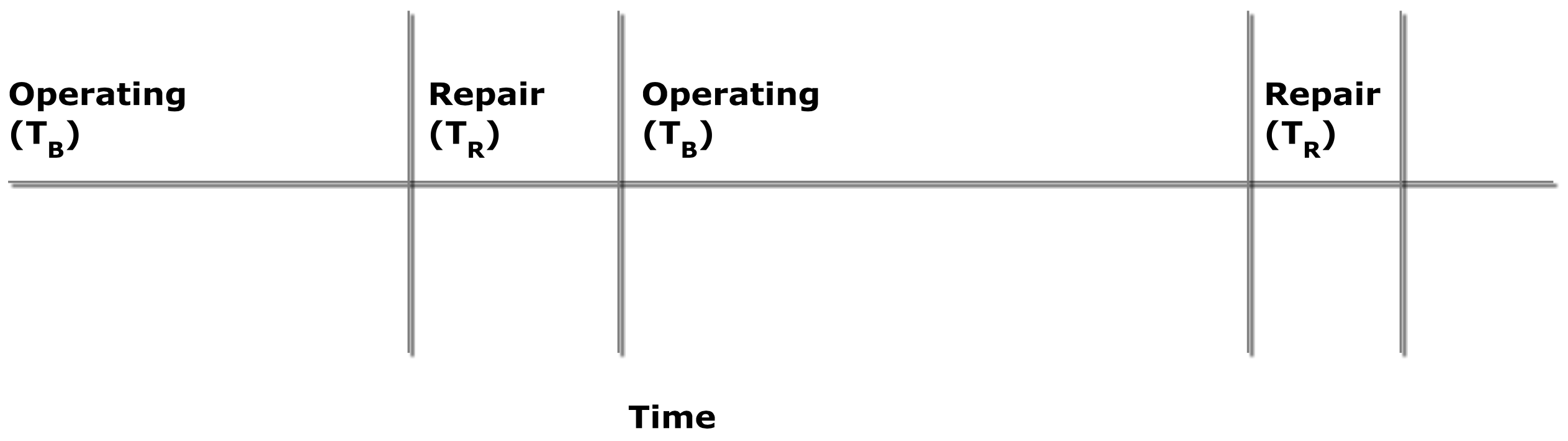
Let T_B denote the average time between the end of a repair and the next breakdown and T_R denote the average repair time. Then the quantity T_B + T_R is the length in time of the breakdown- repair cycle. The availability is defined as the percent of time the machine is not broken and is computed as follows.

\begin{align}A=\frac{T_{B}}{T_{B}+T_{R}}\tag{6-7}\end{align}

The following should be noted concerning availability:

1. The time to complete all work (operations on parts) is reduced to A% of the original time.
2. The lead time for parts waiting for the workstation while it is being repaired will be much longer than for parts that don’t wait for a repair. Thus, the average, maximum, and standard deviation of the lead time will increase.

In this case, the machine breaks down on the average once per week (40 hours) and takes between 30 minutes and 2 hours to repair. Since the time between breakdowns is highly variable, it is modeled as exponentially distributed with a mean of 40 hours. The time to repair is modeled as uniformly distributed between 30 minutes and 2 hours (120 minutes).

The second detractor is defective parts. Either additional parts need to be made or the defective parts need to be reworked to meet the demand. This increases the amount of work that needs to be done to produce the number of parts needed to meet the demand. If additional parts need to be made or the average rework time is the same as the average production time, the number of parts that need to be made is given by equation 6-8 where p is the percent of parts that are defective.

\begin{align}\mathrm{D}_{\mathrm{New}}=\mathrm{D}_{\mathrm{Old}} /(1-\mathrm{p})\tag{6-8}\end{align}

The following should be noted concerning defective parts.

1. The increase in work will increase the utilization of the workstation, which in turn increases the lead time as shown in the VUT equation (6-2).
2. Effectively, there are more arrivals to the workstation which decreases the time between arrivals to TBA * (1-p).

In the case, let p = 5%.

The final detractor is setup and the resulting batching of parts. The setup and batching process is as follows. As they arrive, parts are gathered into a group called a batch until the number of parts in the group equals the predetermined batch size (b). The newly formed batch enters the buffer of the machine to wait processing. Processing the batch means performing a setup operation on the machine and then processing all items in the batch.

The following should be noted concerning setup and batching.

1. Waiting for a batch to form will increase the average, maximum, and standard deviation of lead time.
2. The following must be true: b*takt time >= setup time + b * operation time
3. The minimum feasible batch size may be greater than one, given the preceding item in the list.

This leads to the following question: What is the smallest value of the batch size such that the utilization, which now includes the setup time, is as close as possible to a given value? Decreasing the batch size increases the number of setups and thus the amount of time spent doing setup work, which is not productive. However, decreasing the batch size decreases the work in process and finished goods inventories and supports a more flexible production schedule. These goals are consistent with achieving a lean production environment.

The utilization should be computed as shown in equation 6-9.

\begin{align}\mu=\left(\text { setup time }+\mathrm{b}^{*} \mathrm{CT}\right) /\left(\mathrm{b}^{*} \mathrm{T}_{\mathrm{a}}\right)\tag{6-9}\end{align}

Then the smallest batch size for a given value of the utilization is given by equation 6-9a.

\begin{align}b=\operatorname{setup} \operatorname{time} /\left(u * T_{a}-C T\right)\tag{6-9a}\end{align}

This problem also can be formulated and solved using a spreadsheet to facilitate evaluating alternative values of the batch size. These alternatives could include complying with constraints such as the batch size must be a multiple of 10. The evaluation is done by computing the utilization and number of batches as a function of the selected batch size.

The target utilization is entered. The absolute deviation between the actual utilization and the target is minimized. In other words, the batch size n is changed until the actual utilization is as close as possible to the target. This may be done manually or with one of the spreadsheet tools: solver and goal seek. Note: if goal seek is used, start with a very small batch size.

In this case, the target utilization is set to 95% and the setup time is 30 minutes. Table 6-4 shows the how a batch size of 42 was determined. Note the value of the batch size computed using equation 6-9a is 42.9.

Table 6-4: Result of Finding a Target Batch Size
Inputs	Target Utilization	95%
	Average Time Between Arrivals	6
	CT	5
	Setup Time	30
	Demand	1680
Result	Batch size (b)	42
Computations	Numerator	240
	Denominator	252
	Utilization	95.2%
	Deviation	0.2%
	Number of Batches	40