
7.3: The Case Study
- Page ID
- 30990

In this application study, we consider a serial line where it is essential to minimize buffer space between workstations without compromising lead time.
7.3.1 Define the Issues and Solution Objective
A new three workstation serial line process is being designed for an electronics assembly manufacturing system. The line produces one type of circuit card with some small design differences between cards allowed. The line must meet a lead time requirement that is yet undetermined. Circuit cards are batched into relatively large trays for processing before entering the line.
Only a small amount of space is available in the plant for the new line, so inter-station buffer space must be kept to a minimum. A general storage area with sufficient space can be used for circuit card trays prior to processing at the first workstation. Engineers are worried that the small inter-station buffer space will result in severe blocking that will prevent the lead time target from being reached. The objective is to determine the relationship between buffer size and lead time noting the amount of blocking that occurs. This knowledge will aid management in determining the final amount of buffer space to allocate. Management demands that production requirements be met weekly. Overtime will be allowed if necessary.
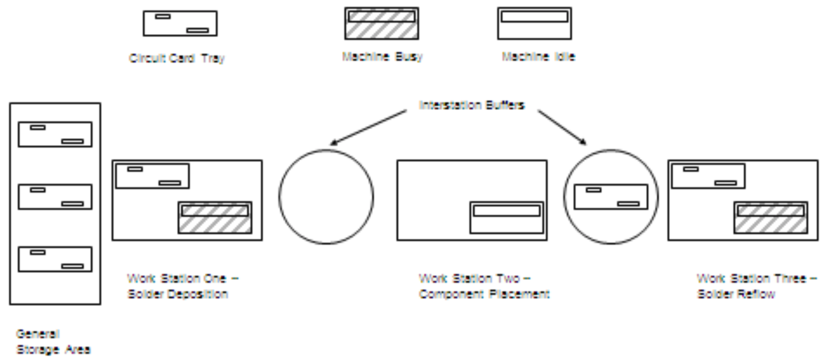
The layout of the line is shown in Figure 7-2. A single circuit card is used to represent a tray. All cards in the tray are processed simultaneously by each machine. Three circuit card trays are shown waiting in the general storage area for the solder deposition station, which is busy. The component placement station is idle and its buffer is empty. The solder reflow station is busy with one circuit card tray waiting.
The time between the arrival of circuit card trays to the first workstation is exponentially distributed with mean 3.0 minutes. The processing time distribution is the same at each workstation: uniformly distributed between 0.7 and 4.7 minutes.1 This indicates that the line is balanced, as it should be.
1 Alternatively, some simulation languages such as Automod express the uniform distribution as mean and half range instead of minimum and maximum. Thus, a uniform distribution between 0.7 and 4.7 can be equivalently expressed as 2.7 ± 2.0.
Figure 7-2: Three station serial system for Electronios Assembly Manufacturing
7.3.2 Build Models
The model of the serial system includes the arrival process for circuit cards, operations at the three stations, and tray movement into and out of the two inter-station buffers.
There are four entity attributes. One entity attribute is arrival time to the system, ArrivalTime. The other three entity attributes store the operation times for that particular entity at each station.
Assigning all operating times when the entity arrives assures that the first entity has the first operating time sample at each station, the second the second and so forth. This assignment is the best way to ensure that the use of common random numbers is most effective in reducing the variation between system alternative scenarios, which aids in finding statistical differences between the cases. In general, the nth arriving entity may not be the nth entity processed at a particular station. In the serial line model, this will be the case since entities can't "pass" each other between stations.
The processing of a circuit card tray at the deposition station is done in the following way. A circuit card tray uses the station when the latter becomes idle. The operation is performed. The circuit card tray then must find a place in the inter-station buffer before leaving the deposition station. Thus, the deposition station enters the blocked state until the circuit card tray that has just been processed enters the inter-station buffer. Then the station enters the idle state. This logic is repeated for the placement station. The tray departs the line following processing at the reflow station.
The pseudo-English for the model follows. Note that there is one process for arriving entities, one for departing entities and one for each of the three workstations.
| // Serial Line Model | |
| Define Arrivals: \(\ \quad\quad\)Time of first arrival: \(\ \quad\quad\)Time between arrivals: \(\ \quad\quad\)Number of arrivals: |
0 Exponentially distributed with a mean of 3 minutes Exponential (3) minutes Infinite |
| Define Resources: \(\ \quad\quad\)WS_Deposition/1 \(\ \quad\quad\)WS_Placement/1 \(\ \quad\quad\)WS_Reflow/1 \(\ \quad\quad\)WS_BufferDP/? \(\ \quad\quad\)WS_BufferPR/? |
with states (Busy, Idle, Blocked) with states (Busy, Idle, Blocked) with states (Busy, Idle) with states (Busy, Idle) with states (Busy, Idle) |
| Define Entity Attributes: \(\ \quad\quad\)ArrivalTime \(\ \quad\quad\)OpTimeDes \(\ \quad\quad\)OpTimePlace \(\ \quad\quad\)OpTimeReflow |
// part tagged with its arrival time; each part has its own tag // operation time at deposition station // operation time at placement station // operation time at reflow station |
| Process Arrive Begin \(\ \quad\quad\)Set ArrivalTime = Clock \(\ \quad\quad\)Set OpTimeDes = uniform(0.7, 4.7)2 \(\ \quad\quad\)Set OpTimePlace = uniform(0.7, 4.7) \(\ \quad\quad\)Set OpTimeReflow = uniform(0.7, 4.7) \(\ \quad\quad\)Send to Process Deposition End |
// record time part arrives on tag // set operations times at each station // start processing |
| Process Deposition // Deposition Station Begin \(\ \quad\quad\)Wait until WS_Deposition/1 is Idle in Queue Q_Deposition \(\ \quad\quad\)Make WS_Depostion/1 Busy \(\ \quad\quad\)Wait for OpTimeDes minutes \(\ \quad\quad\)Make WS_Deposition/1 Blocked \(\ \quad\quad\)Wait until WS_BufferDP/1 is Idle \(\ \quad\quad\)Make WS_Deposition/1 Idle \(\ \quad\quad\)Send to Process Placement End |
// wait its turn on the machine // tray starts turn on machine; machine is busy // tray is processed // tray is finished; machine is Blocked // wait for interstation buffer space // free deposition machine // Send to placement machine |
| Process Placement // Placement Station Begin \(\ \quad\quad\)Wait until WS_Placement/1 is Idle \(\ \quad\quad\)Make WS_BufferDP/1 Idle \(\ \quad\quad\)Make WS_Placement/1 Busy \(\ \quad\quad\)Wait for OpTimePlace minutes \(\ \quad\quad\)Make WS_Placement/1 Blocked \(\ \quad\quad\)Wait until WS_BufferPR/1 is Idle \(\ \quad\quad\)Make WS_Placement/1 Idle \(\ \quad\quad\)Send to Process Reflow End |
// wait its turn on the machine // leave interstation buffer // tray starts turn on machine; machine is busy // tray is processed // tray is finished; machine is Blocked // wait for interstation buffer space // free placement machine // Send to reflow machine |
| Process Reflow // Reflow Station Begin \(\ \quad\quad\)Wait until WS_Reflow1 is Idle \(\ \quad\quad\)Make WS_BufferPR/1 Idle \(\ \quad\quad\)Make WS_Reflow/1 Busy \(\ \quad\quad\)Wait for OpTimeReflow minutes \(\ \quad\quad\)Make WS_Reflow/1 Idle \(\ \quad\quad\)Send to Process Depart End |
// wait its turn on the machine // leave interstation buffer // tray starts turn on machine; machine is busy // tray is processed // free placement machine // Send to reflow machine |
| Process Depart Tabulate (Clock-ArrivalTime) in LeadTime End |
// keep track of part time on machine |
2 In Automod this would be written using the midpoint, half-range style: uniform 2.7, 2.0
7.3.3 Identify Root Causes and Assess Initial Alternatives
The experiment design is summarized in Table 7-1.
| Table 7-1: Simulation Experiment Design for the Serial System | |
| Element of the Experiment | Values for This Experiment |
| Type of Experiment | Terminating |
| Model Parameters and Their Values | Size of each buffer -- (1, 2, 4, 8, 16) |
| Performance Measures3 | 1. Lead Time 2. Percent blocked time depostion station 3. Percent blocked time placement station |
| Random Number Streams | 1. Time between arrivals 2. Operation time deposition station 3. Operation time placement station 4. Operation time reflow station |
| Initial Conditions | 1 circuit card tray in each inter-station buffer with the following station busy |
| Number of Replicates | 20 |
| Simulation End Time | 2400 minutes (one week) |
Since management assesses production weekly, a terminating experiment with a simulation time interval of one week was chosen. The size of each of the two buffers is of interest. Note that the workstations in this study have the same operation time distribution, indicating that the line is balanced as it should be. Analytic and empirical research have shown that for serial systems whose workstations have the same operation time distribution that buffers of equal size are preferred (Askin and Standridge, 1993; Conway et al., 1988).
There was some debate as to whether throughput, WIP, or lead time should be the primary performance measure. Since all circuit card trays that arrive also depart eventually the throughput rate in-bound to the system is the same as the throughput rate out-bound from the system, at least in the long term. Note that by Little's Law, the ratio of the WIP to the lead time (LT) is equal to the (known) throughput rate. Thus, either the total WIP, including that preceding the first workstation, or the lead time could be measured.
3 The problems at the end of the chapter reference the performance measures not discussed in the text.
The lead time is easy to observe since computing it only requires recording the time of arrivals as a entity attribute. Thus, the lead time can be computed when a entity leaves the system. Computing the WIP requires counting the number of entities within the line. This also is straightforward. We will choose to compute the lead time for this study.
Buffer size is the model parameter of interest. The relationship between buffer size and lead time is needed. Thus, various values of buffer size will be simulated and the lead time observed. Average lead time is one performance measure statistic of interest along with the percent blocked time of each station.
There are four random variables in the model, the time between arrivals and three operation times, with one stream for each. The simulated time interval is the same as the management review period for production, one week. Twenty replicates will be made. Since the utilization of the stations is high, a busy station with one circuit card tray in the preceding inter-station buffer seems like a typical system state. Thus, the initial conditions were determined.
Verification and validation evidence were obtained from a simulation experiment with the inter- station buffer size set to the maximum value in the experiment, 16. Results show almost no blocking in this case. Verification evidence consists of balancing the number of arrivals with the number of departures and the number remaining in the simulation at the end of the run for one replicate. These values are shown in Table 7-2.
| Table 7-2: Verification Evidence for Replicate 1 | ||
| Circuit Trays Arriving | Circuit Trays Departing or Remaining at the end of the Simulation | |
| Initial conditions | 6 | |
| Arrival process | 794 | |
| Completed processing | 785 | |
| In buffers | 12 | |
| In processing | 3 | |
| Total | 800 | 800 |
Validation evidence is obtained by comparing the percent busy time of the deposition station as estimated from the simulation results with the expected value computed as follows. The average operation time is (0.7 + 4.7)/2 = 2.7 minutes. The average time between arrivals is 3 minutes. Thus, the expected percent busy time is 2.7 / 3.0 = 90%. The approximate 99% confidence interval for the true percent busy time computed from the simulation results is 86.7 % - 91.7%. Since this interval contains the analytical determined busy time value, validation evidence is obtained.
Since the other stations can be blocked, their percent busy time is not as straightforward to compute analytically. Thus, validation evidence with regard to the deposition and placement stations is more difficult to obtain.
Simulation results for the various values of inter-station buffer capacity will be compared and differences noted. Statistical analysis will be performed to confirm differences that affect what buffer capacity is chosen. Table 7-3 shows the average lead time for each buffer capacity for each replicate as well as summary statistics.
| Table 7-3: Average Lead Time Summary (minutes) | |||||
| Buffer Capacity | |||||
| Replicate | 1 | 2 | 4 | 8 | 16 |
| 1 | 75.4 | 46.3 | 36.6 | 33.9 | 33.2 |
| 2 | 121.3 | 65.7 | 40.9 | 38.2 | 38.1 |
| 3 | 97.7 | 66.8 | 48.6 | 39.6 | 39.4 |
| 4 | 41.5 | 29.9 | 25.1 | 25.0 | 25.0 |
| 5 | 45.8 | 27.5 | 23.6 | 23.5 | 23.5 |
| 6 | 93.7 | 45.8 | 28.9 | 27.9 | 27.9 |
| 7 | 47.1 | 35.6 | 29.1 | 28.2 | 28.2 |
| 8 | 36.5 | 24.6 | 21.8 | 21.7 | 21.7 |
| 9 | 45.2 | 28.5 | 25.3 | 25.0 | 25.0 |
| 10 | 52.1 | 26.7 | 23.6 | 23.1 | 23.1 |
| 11 | 137.2 | 87.4 | 57.6 | 48.8 | 48.8 |
| 12 | 102.6 | 44.9 | 36.1 | 34.1 | 34.1 |
| 13 | 70.6 | 41.3 | 28.8 | 26.9 | 26.9 |
| 14 | 44.7 | 33.9 | 26.9 | 25.5 | 25.5 |
| 15 | 97.4 | 54.6 | 35.0 | 30.9 | 30.4 |
| 16 | 46.9 | 29.9 | 27.1 | 26.4 | 26.4 |
| 17 | 39.1 | 31.6 | 28.5 | 27.2 | 27.2 |
| 18 | 95.9 | 69.7 | 51.6 | 43.4 | 43.4 |
| 19 | 28.7 | 23.5 | 21.9 | 21.9 | 21.9 |
| 20 | 80.2 | 44.5 | 35.0 | 34.0 | 34.0 |
| Average | 70.0 | 42.9 | 32.6 | 30.3 | 30.2 |
| Std. Dev. | 31.5 | 17.7 | 10.2 | 7.5 | 7.5 |
| 99% CI Lower Bound | 49.8 | 31.6 | 26.1 | 25.5 | 25.4 |
| 99% CI Upper Bound | 90.2 | 54.3 | 39.1 | 35.1 | 35.0 |
Figure 7-3 shows a graph of the average time in the system versus the buffer capacity. From Table 7-3 and Figure 7-3 it is easily seen that the average time in the system decreases significantly when the buffer capacity is increased from 1 to 2 as well as from 2 to 4. Smaller decreases are seen when the buffer capacity is increased further. The statistical significance of these latter differences will be determined.
Figure 7-3: Average Time in the System versus Buffer Capacity
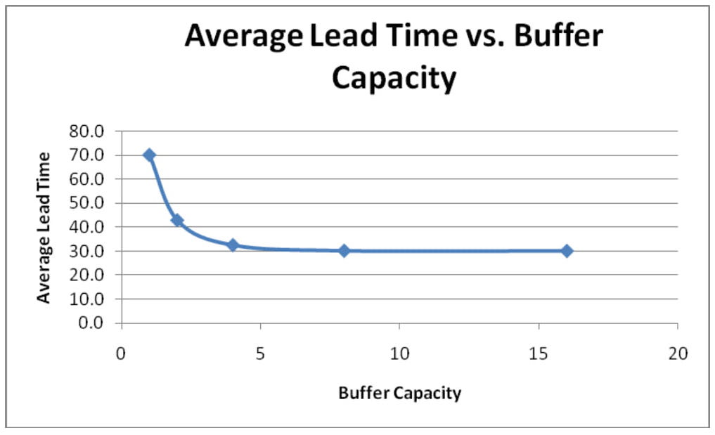
The minimum possible average time in the system is the sum of the average processing times at each station 2.7 + 2.7 + 2.7 = 8.1 minutes. Note that for buffer sizes of 4, 8, and 16, the average time in the system is 4 to 5 times the minimum average cycle time. This is due to the high degree of variability in the system: exponential arrival times and uniformly distributed service times with a wide range as well as the high utilization of the work stations. This result is consistent with the VUT equation that shows that the lead time increases as the variability of the time between arrivals, the variability of the service time, and the utilization increase.
The paired-t method is used to compute approximate 99% confidence intervals for the average difference in lead time for selected buffer sizes. These results along with the approximate 99% confidence intervals for the average lead time for each buffer size are shown in Table 7-4. Note that average lead time reduction using 16 buffers instead of 8, is not statistically significant since the approximate 99% confidence interval for the difference in average lead time contains 0.
Table 7-5 summarizes the percent blocked time for the deposition station as well as the differences in percent block time including paired-t confidence intervals for the mean difference for neighboring values of buffer sizes of interest.
The percentage of time that the deposition station is blocked decreases as the buffer size increases as would be expected. The paired-t confidence interval for the difference in percentage of blocked time for 16 buffers versus 8 buffers does not contain 0. Thus, the reduction in percent blocked time due to the larger buffer size is not statistically significant. Further note that the 99% confidence intervals for the percent of time blocked for the case of 8 and 16 buffers both contain 0. Thus, the percent of blocked time for these cases is not significantly different from zero.
| Table 7-4: Paired t Test for Average Lead Time (minutes) | |||||
| Buffer Capacity | |||||
| Replicate | 4 | 8 | Diff4-8 | 16 | Diff 8 -16 |
| 1 | 36.6 | 33.9 | 2.7 | 33.2 | 0.7 |
| 2 | 40.9 | 38.2 | 2.7 | 38.1 | 0.1 |
| 3 | 48.6 | 39.6 | 9.0 | 39.4 | 0.3 |
| 4 | 25.1 | 25.0 | 0.2 | 25.0 | 0.0 |
| 5 | 23.6 | 23.5 | 0.1 | 23.5 | 0.0 |
| 6 | 28.9 | 27.9 | 0.9 | 27.9 | 0.0 |
| 7 | 29.1 | 28.2 | 0.9 | 28.2 | 0.0 |
| 8 | 21.8 | 21.7 | 0.1 | 21.7 | 0.0 |
| 9 | 25.3 | 25.0 | 0.4 | 25.0 | 0.0 |
| 10 | 23.6 | 23.1 | 0.5 | 23.1 | 0.0 |
| 11 | 57.6 | 48.8 | 8.9 | 48.8 | 0.0 |
| 12 | 36.1 | 34.1 | 2.0 | 34.1 | 0.0 |
| 13 | 28.8 | 26.9 | 1.9 | 26.9 | 0.0 |
| 14 | 26.9 | 25.5 | 1.4 | 25.5 | 0.0 |
| 15 | 35.0 | 30.9 | 4.1 | 30.4 | 0.5 |
| 16 | 27.1 | 26.4 | 0.7 | 26.4 | 0.0 |
| 17 | 28.5 | 27.2 | 1.3 | 27.2 | 0.0 |
| 18 | 51.6 | 43.4 | 8.2 | 43.4 | 0.0 |
| 19 | 21.9 | 21.9 | 0.0 | 21.9 | 0.0 |
| 20 | 35.0 | 34.0 | 1.0 | 34.0 | 0.0 |
| Average | 32.6 | 30.3 | 2.34 | 30.2 | 0.08 |
| Std. Dev. | 10.2 | 7.5 | 2.92 | 7.5 | 0.19 |
| 99% CI Lower Bound | 26.1 | 25.5 | 0.47 | 25.4 | >-0.04 |
| 99% CI Upper Bound | 39.1 | 35.1 | 4.21 | 35.0 | 0.21 |
| Table 7-5: Paired-t Confidence Intervals for Deposition Percent Blocked Time | |||||
| Buffer Capacity | |||||
| Replicate | 4 | 8 | Diff4-8 | 16 | Diff 8 -16 |
| 1 | 2.51% | 1.11% | 1.41% | 0.00% | 1.11% |
| 2 | 1.57% | 0.00% | 1.57% | 0.00% | 0.00% |
| 3 | 1.12% | 0.29% | 0.83% | 0.00% | 0.29% |
| 4 | 0.84% | 0.00% | 0.84% | 0.00% | 0.00% |
| 5 | 0.53% | 0.00% | 0.53% | 0.00% | 0.00% |
| 6 | 1.48% | 0.11% | 1.37% | 0.00% | 0.11% |
| 7 | 2.19% | 0.00% | 2.19% | 0.00% | 0.00% |
| 8 | 0.69% | 0.00% | 0.69% | 0.00% | 0.00% |
| 9 | 0.66% | 0.10% | 0.56% | 0.00% | 0.10% |
| 10 | 0.49% | 0.00% | 0.49% | 0.00% | 0.00% |
| 11 | 3.62% | 1.65% | 1.96% | 0.20% | 1.45% |
| 12 | 0.90% | 0.00% | 0.90% | 0.00% | 0.00% |
| 13 | 0.61% | 0.00% | 0.61% | 0.00% | 0.00% |
| 14 | 1.33% | 0.12% | 1.21% | 0.00% | 0.12% |
| 15 | 1.46% | 0.12% | 1.33% | 0.00% | 0.12% |
| 16 | 1.30% | 0.29% | 1.01% | 0.00% | 0.29% |
| 17 | 0.69% | 0.16% | 0.53% | 0.00% | 0.16% |
| 18 | 2.74% | 1.26% | 1.47% | 0.17% | 1.09% |
| 19 | 0.66% | 0.10% | 0.57% | 0.00% | 0.10% |
| 20 | 2.35% | 0.42% | 1.92% | 0.00% | 0.42% |
| Average | 1.39% | 0.29% | 1.10% | 0.02% | 0.27% |
| Std. Dev. | 0.87% | 0.48% | 0.53% | 0.06% | 0.43% |
| 99% CI Lower Bound | -0.02% | 0.76% | -0.02% | -0.01% | |
| 99% CI Upper Bound | 0.59% | 1.44% | 0.06% | 0.54% | |
7.3.4 Review and Extend Previous Work
System experts reviewed the results developed
buffer size of four should be used in the system. The small, approximately 10%, decrease in average lead time obtained with a buffer size of 8 did not justify the extra space. The difference was statistically significant in the simulation experiment. The average percent blocked time for the deposition station is about 1.4% percent for a buffer size of 4.
It was noted that for some replicates the average lead time was near an hour. This was of some concern.
7.3.5 Implement the Selected Solution and Evaluate
The system was implemented with 4 buffers. Average lead will be monitored. Causes of long average lead time will be identified and corrected.