8.3: The Case Study

This case study deals with determining the number of machines needed at each workstation to meet a particular level of demand with a satisfactory service level. The average number of busy machines can be determines using Little's law. However, due to waiting time for busy machines, lead time may exceed management's target. In other words, the service level is too low. Additional machines at a station reduce utilization and thus reduce lead time.

8.3.1 Define the Issues and Solution Objective

A job shop consists of four workstations each having one kind of machine: lathe, planer, shaper, and polisher as shown in Figure 8-1. There is one route through the job shop for each of the three job types. Machines may be either in a busy or idle state.

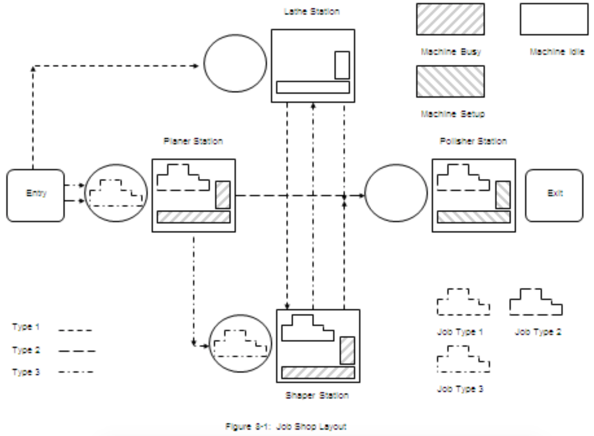
Management desires that each job spends less than 8 hours in the shop. The service level is the percent of jobs that meet this target. The objective is to find the minimum number of machines, and thus capital equipment cost, that allows the shop to reach a high, but yet unspecified service level. Management reviews shop performance each month.

The shop processes three types of jobs that have the following routes through the shop:

Type 1: lathe, shaper, polisher
Type 2: planer, polisher
Type 3: planer, shaper, lathe, polisher

Each type of job has its own arrival process, that is its own distribution of time between arrivals. Job processing time data was not available by job type. Thus, a single distribution is used to model operation time at a station. Setup issues can be ignored for now.

Relevant data are as follows. The time between arrivals for each job type is exponentially distributed. The mean time between arrivals for job type 1 is 2.0 hours, for type 2 jobs 2.0 hours, and for type 3 jobs 0.95 hours. Processing times are triangularly distributed with the following parameters (minimum, mode, maximum), given in hours.

Planer: (1.0, 1.2, 2.4)

Shaper: (0.75, 1.0, 2.0)

Lathe: (0.40, 0.80, 1.25)

Polisher: (0.5, 0.75, 1.5)

8.3.2 Build Models

The model of the job shop uses the following logic:

1. A job arrives as modeled in the arrival process.
2. The job is routed according to the routing process.
   1. If the job needs more operations, it is sent to the station corresponding to its next operation.
   2. If the job has completed all operations, its lead time is computed and the service level for this job recorded. Then the job leaves the shop. Note that the service level is either 100 for acceptable (less than 8 hours) or 0 for not acceptable (greater than 8 hours).
3. The job is processed at the selected workstation as modeled by an operation process.
4. The job returns to step 2.

Job routing corresponds to the routing matrix shown in Figure 8-2, with Depart indicating that the end of the route has been reached.

Job Type	First Operation	Second Operation	Third Operation	Fourth Operation	Last
1	Lathe	Shaper	Polisher	Depart
2	Planer	Polisher	Depart
3	Planer	Shaper	Lathe	Polisher	Depart

Figure 8-2. Job Shop Routing Matrix.

Enitities represent jobs and have the following attributes:
JobType =	type of job
ArriveTime =	simulation time of arrival
Location =	location of a job relative to the start of its route: 1st..4th
OpTimei =	operation time at the ith station on the route of a job: i = 1..4
Routei =	station at the ith location on the route of a job
ArriveStation =	time of arrival to a station, used in computing the waiting time at a station

There is an arrival process for each job type. The arrival processes for the job types are similar. All of the attributes are assigned including each operation time. The operation time is assigned to assure that the ith arriving job (entity) will be assigned the ith sample from each random number stream for each alternative tested. This is the best implementation of the common random numbers method discussed in chapter 4. The values assigned to the Route attribute are the names of the stations that comprise the route in the order visited. The last station is called Depart to indicate that the entity has completed processing. Whatever performance measure observations are needed are made in the Depart process. At the end of the arrival process, the entity is sent to the routing process.

The routing process is as follows. The Location relative to the start of the route is incremented by 1. The entity is sent to the process whose name is given by Route_Location. The routing process requires zero simulation time.

The process as each station is like that of the single workstation discussed in chapter 6. An arriving entity waits for the planer resource. The operation is performed and the resource is made idle. The entity is sent to the routing process.

The pseudo-English form of the model including the arrival process for type 1 jobs, the operation process for the planer, the routing process and the depart process follows.

---

Define Arrivals: \(\ \quad\quad\)Type1 \(\ \quad\quad\quad\quad\)Time of first arrival: \(\ \quad\quad\quad\quad\)Time between arrivals: \(\ \quad\quad\)Type2 \(\ \quad\quad\quad\quad\)Time of first arrival: \(\ \quad\quad\quad\quad\)Time between arrivals: \(\ \quad\quad\)Type3 \(\ \quad\quad\quad\quad\)Time of first arrival: \(\ \quad\quad\quad\quad\)Time between arrivals:	0 Exponentially distributed with a mean of 2 hours Number of arrivals: Infinite 0 Exponentially distributed with a mean of 2 hours Number of arrivals: Infinite 0 Exponentially distributed with a mean of 0.95 hours Number of arrivals: Infinite
Define Resources: \(\ \quad\quad\)Lathe/? \(\ \quad\quad\)Planer/? \(\ \quad\quad\)Polisher/? \(\ \quad\quad\)Shaper/?	with states (Busy, Idle) with states (Busy, Idle) with states (Busy, Idle) with states (Busy, Idle)
Define Entity Attributes: \(\ \quad\quad\)ArrivalTime \(\ \quad\quad\)JobType \(\ \quad\quad\)Location \(\ \quad\quad\)OpTime(4) \(\ \quad\quad\)Route(5) \(\ \quad\quad\)ArriveStation	// part tagged with its arrival time; each part has its own tag // type of job // location of a job relative to the start of its route: 1..4 // operation time at the ith station on the route of a job // station at the ith location on the route of a job // time of arrival to a station, used in computing the waiting time
Process ArriveType1 Begin \(\ \quad\quad\)Set ArrivalTime = Clock \(\ \quad\quad\)Set Location = 0 \(\ \quad\quad\)Set JobType = 1 \(\ \quad\quad\)// Set route and processing times \(\ \quad\quad\)Set Route(1) to Lathe \(\ \quad\quad\)Set OpTime(1) to triangular 0.40, 0.80, 1.25 hr \(\ \quad\quad\)Set Route(2) to Shaper \(\ \quad\quad\)Set OpTime(2) to triangular 0.75, 1.00, 2.00 hr \(\ \quad\quad\)Set Route(3) to Polisher \(\ \quad\quad\)Set OpTime(3) to triangular 0.50, 0.75, 1.50 hr \(\ \quad\quad\)Set Route(4) to End \(\ \quad\quad\)Send to P_Route End	// record time job arrives on tag // job at start of route
Process Planer Begin \(\ \quad\quad\)Set ArriveStation = Clock \(\ \quad\quad\)Wait until Planer/1 is Idle in Queue QPlaner \(\ \quad\quad\)Make Planer/1 Busy \(\ \quad\quad\)Tabulate (Clock-ArriveStation) in WaitTimePlaner \(\ \quad\quad\)Wait for OpTime(Location) hours \(\ \quad\quad\)Make Planer/1 Idle \(\ \quad\quad\)Send to P_Route End	// record time job arrives at station // job waits for its turn on the machine // job starts on machine; machine is busy // keep track of job waiting time // job is processed // job is finished; machine is idle
Process Route Begin \(\ \quad\quad\)Location++ \(\ \quad\quad\)Send to Route(Location) End	// Increment location on route // Send to next station or depart
Process Depart Begin //Lead time in hours by job type and for all job types if type = Job1 then tabulate (Clock-ArrivalTime) in LeadTime(1) if type = Job2 then tabulate (Clock-ArrivalTime) in LeadTime(2) if type = Job3 then tabulate (Clock-ArrivalTime) in LeadTime(3) tabulate ((Clock-ArrivalTime) in LeadTimeAll if ((Clock-ArrivalTime) <= 8 tabulate 100 in Service else tabulate 0 in Service End	// Service level recorded

---

8.3.3 Identify Root Causes and Assess Initial Alternatives

Management reviews the system monthly. Thus, a terminating experiment with an ending time of one month was chosen. Furthermore, management is interested in the percent of jobs that spend less than 8 hours in the shop, the service level, as well as job waiting time at each station. These quantities are the performance measures of interest.

There are seven random number streams, one for the arrival process for each of three types of jobs and one for each of four operation times. Twenty replicates will be made. The initial conditions reflect a typical state of the shop: two jobs of each type at each station.

The model parameters are the number of machines at each station. The expected number of busy machines at each station will be used as the parameter value for the first simulation. Management is able to provide more machines at workstations where the maximum waiting time is excessive in order to meet the service level target.

Table 8-1 summarizes the simulation experiment.

Table 8-1: Simulation Experiment Design for the Job Shop
Element of the Experiment	Values for This Experiment
Type of Experiment	Terminating
Model Parameters and Their Values	Number of machines at each station: 1. Average number busy as shown in Table 8-2 following
Performance Measures	1. Percent of jobs whose cycle time is less than 8 hours (Service Level) 2. Waiting time at each station
Random Number Streams	1. Time between arrivals - job type 1 2. Time between arrivals - job type 2 3. Time between arrivals - job type 3 4. Operation time station 1 5. Operation time station 2 6. Operation time station 3 7. Operation time station 4
Initial Conditions	2 parts of each type that can be at a station in the buffer of each station
Number of Replicates	20
Simulation End Time	184 hours (one month)

The expected number of machines needed by each part type at each station is computed as shown in Table 8-2.

1. The mean service time is the mean of the triangular distribution of the service time at each station. This quantity is the arithmetic average of the minimum, mode, and maximum.
2. The expected number of machines is the quotient of the mean operation time divided by the mean time between arrivals (Little's Law).
3. The total expected number of machines at a station is the sum over the three part types. This value is rounded to the next higher whole number to yield the number of machines at each station.
4. Raw processing time is the sum of the mean processing times at each station on the route of a job.

Table 8-2: Expected Number of Machines Needed at Each Workstation
	Planer	Shaper	Lathe	Polisher	Raw Processing Time
Job Type 1
Mean Time Between Arrivals (TBA = 1/TH)		2	2	2
Mean Operation Time (CT)		1.25	0.82	0.92	2.99
Expected Number of Machines (= CT / TBA)		0.63	0.41	0.46
Job Type 2
Mean Time Between Arrivals (TBA)	2			2
Mean Operation Time (CT)	1.53			0.92	2.45
Expected Number of Machines (= CT / TBA)	0.77			0.46
Job Type 3
Mean Time Between Arrivals (TBA)	0.95	0.95	0.95	0.95
Mean Operation Time (CT)	1.53	1.25	0.82	0.92	4.52
Expected Number of Machines (= ST / TBA)	1.61	1.32	0.86	0.97
Total Expected Number of Machines	2.38	1.94	1.27	1.89
Number of Machines to Use	3	2	2	2

The mean raw processing time for the job types are 1.45 hours, 2.99 hours, and 4.52 hours. Thus, a cycle time in the shop criteria of one day (8 hours) represents approximate 2 to 5 times the raw processing time which seems reasonable.

Table 8-3 gives the service level for the shop and the maximum waiting time at each station. Notice that the service level is highly variable, ranging from 19.8% to 97.3%. Maximum waiting times are much larger for the shaper than any of the other three machines. The maximum waiting times at the polisher and the planer are also long.

Table 8-3: Simulation Results - Expected Number of Machines Case.
Replicate	Service Level	Maximum Waiting Time at the Lathe (Hours)	Maximum Waiting Time at the Planer (Hours)	Maximum Waiting Time at the Polisher (Hours)	Maximum Waiting Time at the Shaper (Hours)
1	21.2	1.1	4.4	4.6	23.0
2	42.7	1.6	3.3	4.0	10.7
3	22.8	1.2	8.6	9.8	17.1
4	40.1	1.4	5.1	3.4	11.2
5	97.3	1.0	2.6	3.4	2.8
6	73.4	0.8	5.0	4.4	4.4
7	62.4	2.2	2.9	2.8	13.9
8	74.0	1.5	3.9	4.0	9.1
9	24.7	2.2	4.1	4.9	14.0
10	37.6	1.3	4.8	3.3	13.0
11	57.8	1.5	3.6	3.4	7.8
12	19.8	1.1	8.8	9.2	13.3
13	38.0	1.1	7.0	3.7	10.0
14	70.8	1.0	3.1	4.2	9.0
15	36.9	1.1	4.1	6.5	11.5
16	76.2	1.1	3.1	3.5	8.3
17	59.3	1.0	3.0	6.0	7.9
18	60.6	1.5	5.3	4.5	6.3
19	31.1	1.4	3.8	9.1	7.0
20	24.4	1.1	5.3	4.5	16.8
Average	48.6	1.3	4.6	5.0	10.9
Std. Dev.	22.5	0.4	1.8	2.1	4.7
99% CI Lower Bound	34.2	0.1	0.4	0.5	1.1
99% CI Upper Bound	62.9	2.9	2.9	2.9	2.9

8.3.4 Review and Extend Previous Work

System experts reviewed the results developed in the previous section. The average service level of 48.6% was thought to be too low. A service level of at least 95% is needed. A machine will be added to the the shaper station to reduce the maximum waiting time. Additional machines will be added one at a time to the station with the greatest maximum waiting time until the 95% service level is achieved.