9.4: Introduction to Pull Inventory Management

The inventor of just-in-time manufacturing, Taiichi Ohno, defined the term pull as follows:

Manufacturers and workplaces can no longer base production on desktop planning alone and then distribute, or push, them onto the market. It has become a matter of course for customers or users, each with a different value system, to stand in the frontline of the marketplace and, so to speak, pull the goods they need, in the amount and at the time they need them.

A supermarket (grocery store) has long been a realization of a pull system. Consider a shelf filled with cans of green beans. As customers purchase cans of green beans, less cans remain on the shelf. The staff of the grocery store restocks the shelf whenever too few cans remain. New cans are taken from boxes of cans in the store room. Whenever the number of boxes of cans in the store room becomes too few, additional boxes are ordered from the supplier of green beans.

Note than in this pull system, shelves are restocked and consequently new cases of green beans are ordered depending on the number of cans on the shelves. The number of cans on the shelves depends on current customer demand for green beans.

The alternative to a pull system, which is no longer commonly used, is a push system. In a push system supermarket, the manager would forecast customer demand for green beans for the next time period, say a month. The forecasted number of green beans would be ordered from the supplier. The allocated shelf space would be stocked with cans of green beans. If actual customer demand was less than the forecasted demand, the manager would need to have a sale to try to sell the excess cans of green beans. If the actual demand was greater than the forecasted demand, the manager would somehow need to acquire more green beans.

This illustration points out one fundamental breakthrough of lean manufacturing: inventory levels, both work-in-process (WIP) and finished goods, are controlled characteristics of how a production system operates instead of a result of how it operates as in a push system.

9.4.1 Kanban Systems: One Implementation of the Pull Philosophy

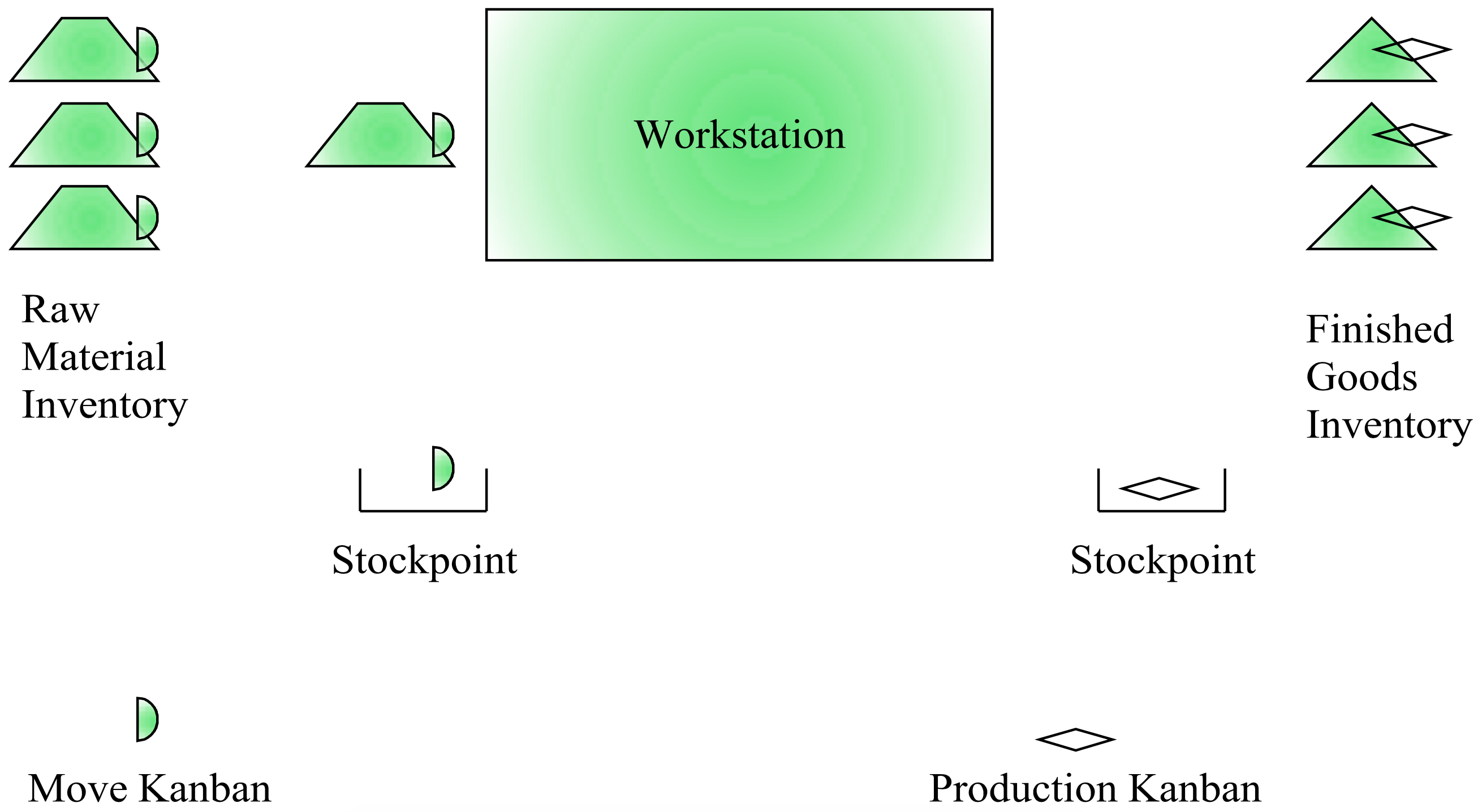
The most common implementation of the pull philosophy is kanban systems. The Japanese word kanban is usually translated into English as card. A kanban or card is attached to each part or batch of parts (tote, WIP rack, shelf, etc.). To understand the significance of such cards, consider a single workstation followed by a finished goods inventory and proceeded by a raw materials inventory as shown in Figure 9- 3. The following items shown in Figure 9-3 are specific to kanban systems.

1. A move kanban shown as a half-moon shaped card attached to the items in the raw material inventory.
2. A production kanban shown as diamond shaped card attached to the items in the finished goods inventory.
3. Stockpoints: locations where kanbans are stored after removal from an item.

The dynamics of this kanban system are as follows.

1. A customer demand causes an item to be removed from the finished goods inventory. The item is given to the customer and the diamond shaped kanban attached to the item is placed in the stockpoint near the finished goods inventory.
2. Periodically, the diamond shaped kanbans are collected from the stockpoint and moved to the workstation. The workstation must produce exactly one item for each diamond shaped kanban it receives. Thus, the finished goods inventory is replenished. Note only the inventory removed by customers is replaced.
3. In order to produce a finished goods item, the workstation must use a raw material item. The workstation receives a raw material item by taking a half-moon shaped kanban to the raw material inventory.

Note the following characteristics of a kanban system.

1. The amount of inventory in a kanban system is proportional to the number of kanbans in the system.
2. Kanban cards and parts flow in oppose directions. Kanbans flow from right to left and parts flow from left to right.
3. The amount of finished goods inventory required depends on the time the workstation takes to produce a part and customer demand. A lower bound on the finished goods inventory can be set given a customer service level, the expected time for the workstation to produce a part, and the probability distribution used to model customer demand.

Figure 9-3: Single Workstation Kanban System

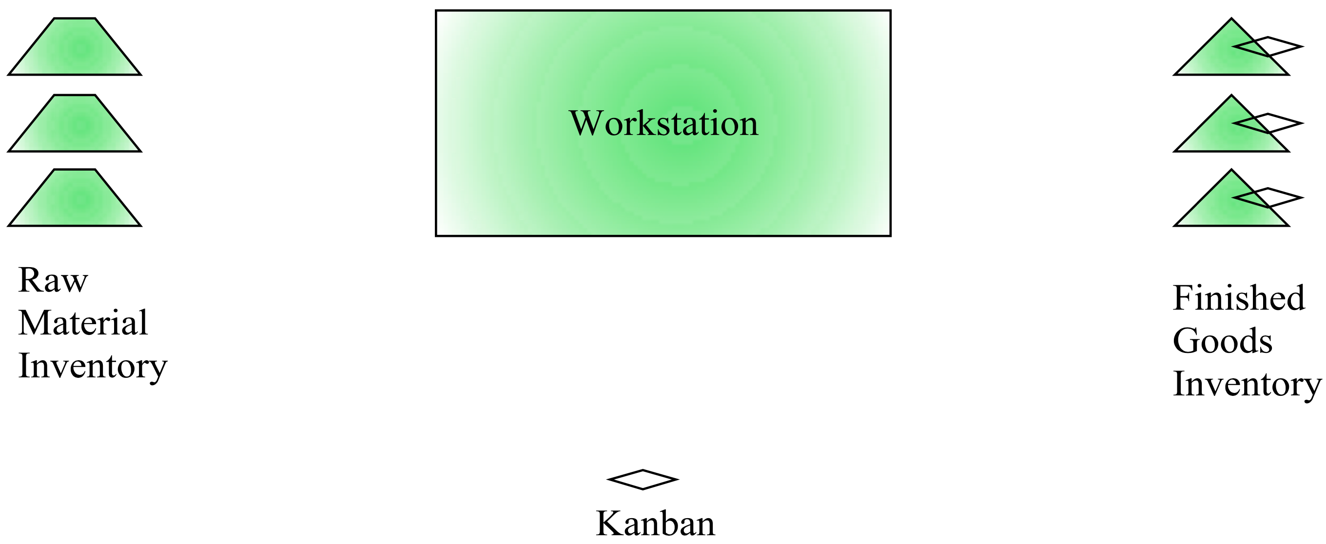
Kanban systems can be implemented in a variety of ways. As a second illustration, consider a modified version of the single workstation kanban system. Suppose only one kanban type is used and information is passed electronically. Such a system is shown in Figure 9-4 and operates as follows:

1. A customer demands an item from the finished goods inventory. The kanban is removed from the item and sent to the workstation immediately.
2. The workstation takes the kanban to the raw material inventory to retrieve an item. The kanban is attached to the item.
3. The workstation processes the raw material into the finished good.
4. The item with the kanban attached is taken to the finished goods inventory.

The number of kanbans can be set using standard methods for establishing inventory levels that have been previously discussed. Try the following problems.

1. Demand for finished goods is Poisson distributed at the rate of 10 per hour. Once an item has been removed from finished goods inventory, the system takes on the average 30 minutes to replace it. How much finished goods inventory should be maintained for a 99% service level?
2. Suppose for problem 1, the time in minutes to replace the inventory is distributed as follows: (30, 60%; 40, 30%; 50, 10%). How much inventory should be kept in this application?
3. Suppose for problem 1, all inventory is kept in containers of size 4 parts. There is one kanban per container. How many kanbans are needed for this situation?

Simulation of a kanban system is discussed in the next chapter.

Figure 9-4: Single Workstation Kanban System -- One Kanban Type

9.4.2 CONWIP Systems: A Second Implementation of the Pull Philosophy

One simple way to control the maximum allowable WIP in a production area is to specify its maximum value. This can be accomplished by using a near constant work-in-process system, or CONWIP system. A production area could be a single station, a set of stations, an entire serial line, an entire job shop, or an entire work cell.

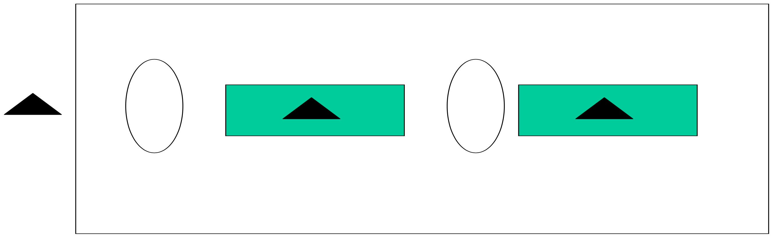
Figure 9.5 shows a small CONWIP system with maximum number of jobs in the production area equal to 2. The rectangle encloses the production system that is under the CONWIP control. Two jobs are in processing, one at each workstation. Thus, the third job cannot enter the production system due to the CONWIP control limit of 2 jobs on the production line even though there is space for the job in the buffer of the first workstation. This job should be waiting in an electronic queue of orders as opposed to occupying physical space outside of the CONWIP area.

Figure 9-5: CONWIP System Illustration

The following are some important characteristics or traits of a CONWIP system.

1. The CONWIP limit is the only parameter of a CONWIP system.
   1. This parameter must be greater than or equal to the number of workstations in the production area. If not, at least one of the workstations will always be starved.
   2. The ideal CONWIP limit is the smallest value that does not constrain throughput.
   3. In a multiple product production area, each job, regardless of type, counts toward the capacity imposed by the single CONWIP limit.
2. A CONWIP system controls the maximum WIP in a production area.
   1. The maximum amount of waiting space before any work station is equal to the CONWIP limit or less. It is possible, but unlikely, that all jobs are at the same station at the same time. Thus, buffer sizes before workstations are usually not a constraint on system operation.
   2. If defective parts are detected at the last station on a production line, the CONWIP limit is the upper bound on the number of defective parts produced.
   3. A smaller footprint is needed for WIP storage.
3. Jobs waiting to enter a production area are organized on an electronic or paper list. No parts are waiting.
   1. The list can be re-ordered as needed so that the highest priority jobs are always at the head of the list. For example, if an important customer asks for a rush job it can always be put at the head of the list. The most number of jobs preceding the highest priority job is given by the CONWIP limit.
   2. If the mix of jobs changes, the CONWIP system dynamically adapts to the mix since the system has only one parameter.
   3. Recall Little's Law: WIP = LT * TH. In CONWIP system, WIP is almost constant. Thus, the lead time to produce is easy to predict given a throughput (demand) rate. With the WIP level controlled, the variability in the cycle time is reduced.
4. For a given value of throughput, the average and maximum WIP level in a CONWIP system is less than in a non-CONWIP (push) system.
5. In a CONWIP system, machines with excess capacity will be idle a noticeable amount of the time, which makes some managers very nervous and makes balancing the work between stations more important.
6. Some CONWIP systems arise naturally as result of the material handling devices employed. For example, the amount of WIP may be limited by the number racks or totes available in the production area.

A simulation model of a CONWIP control would include two processes: one for entering the CONWIP area and one for departing the CONWIP area as shown in the following.

---

CONWIP Processes
Define State Variables: \(\ \quad \quad\)CONWIPLimit \(\ \quad \quad\)CONWIPCurrent	// Number of items allowed in CONWIP area // Number of items currently in CONWIP area
EnterCONWIPArea Process Begin \(\ \quad \quad\)Wait until CONWIPCurrent < CONWIPLimit \(\ \quad \quad\)CONWIPCurrent++ End	// Wait for a space in the CONWIP area // Add 1 to number in CONWIP area
Leave CONWIPArea Process Begin \(\ \quad \quad\)CONWIPCurrent-- End	// Give back space in CONWIP Area

---

Consider the average lead time of jobs in a production area with M workstations. Each workstation has process time t_j. Then the average total processing time is given by summing the average processing times for all work stations yielding the raw processing time, equation 9-15.

\begin{align}t_{p}=\sum_{j=1}^{M} t_{j}\tag{9-15}\end{align}

Suppose the following:

1. The CONWIP limit is set at N\(\ \geq\) M.
2. The production area is balanced, that is the processing time at each station is about the same.
3. Processing times are near constant.

Then the following are true:

1. On the average at each workstation, a job will wait for \(\ \frac{N-M}{M}\) other jobs. M jobs are in processing, one at each station. Thus N-M jobs must be waiting for processing. It is equally likely that a job will be at any station. Thus, the average number of jobs waiting at any station is given by the above quantity.
2. The average waiting time at any particular station is: \begin{align}\left(\frac{N-M}{M}\right) t_{j}\tag{9-16}\end{align}
3. The total lead time at each station is: \begin{align}\left(\frac{N-M}{M}\right) t_{j}+t_{j}=\left(1+\frac{N-M}{M}\right) t_{j}=\left(\frac{N}{M}\right) t_{j}\tag{9-17}\end{align}

Suppose instead that processing times are random and exponentially distributed. This is for practical purposes the practical worst case processing time since c_T = 1.

Then the following are true:

1. On the average at each workstation, a job will wait for \(\ \frac{N-1}{M}\) other jobs. The other N -1 jobs are each equally likely to be at any workstation.
2. The average waiting time at each station is: \begin{align}\left(\frac{N-1}{M}\right) t_{j}\tag{9-18}\end{align}
3. The total lead time at each station is: \begin{align}\left(\frac{N-1}{M}\right) t_{j}+t_{j}=\left(1+\frac{N-1}{M}\right) t_{j}\tag{9-19}\end{align}

9.4.3 POLCA: An Extension to CONWIP

Suri (2010) proposes the Paired-cell Overlapping Loops of Cards with Authorization (POLCA) approach to control the maximum allowable WIP for jobs processed by any pair of Quick Response Manufacturing (QRM) cells. POLCA can be viewed as an extension of CONWIP and is illustrated in Figure 9.6.

Figure 9-6: POLCA Illustration

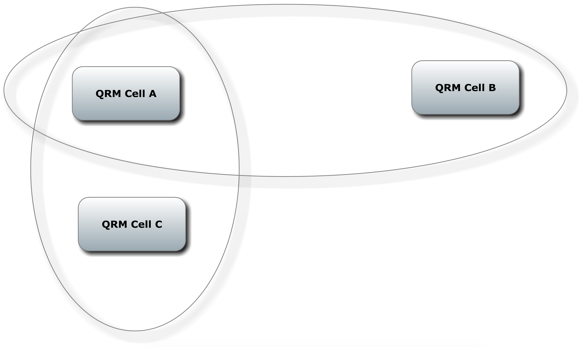
In Figure 9-6, there are two types of jobs: 1) those that are processed by QRM Cell A and QRM Cell B (A- B jobs) as well as 2) those that are processed by QRM Cell A and QRM Cell C (A-C jobs). The WIP for each type of job is controlled separately. There is one maximum WIP value for A-B jobs and a second maximum WIP value for A-C jobs. Thus, there are A-B cards in the system and A-C cards in the system.

To start processing a job, two criteria must be met.

1. There is a card available for that job type, i.e. an A-B card for an A-B job, similar to CONWIP.
2. The current date is at or after the projected start date for the job. The start date is computed as the delivery date minus the allowed time to complete the job.

The card is released for reuse when the job is completed in the second of the pair of cells. That is an A-B card must be acquired before the job starts processing in QRM cell A and is released upon completion of processing in QRM cell B.

The time allowed to complete the job could be determined by expert opinion, experience, the VUT equation or simulation.

Suri suggests estimating the number of POLCA cards needed using Little's Law.

WIP = LT * TH

WIP = # of POLCA cards

LT = Lead time in the first QRM cell + Lead time in the second QRM Cell

TH = Demand rate for jobs for example the number of jobs required per week.

For example, if the average lead time in QRM cell A is 30 minutes, the average lead time in QRM cell B is 25 minutes, the demand per day is 30 units, and the working day is 16 hours then the number of A-B POLCA cards needed is as follows:

LT = (30 + 25)/60 = 0.92 hours

TH = 30/16 = 1.875 units per hour

Number of A-B POLCA cards = LT * TH = 2

The following are some important characteristics or traits of a POLCA system.

7. The POLCA limits are the only parameters of a POLCA system.
   1. If each of the QRM cells in a pair has only one POLCA card type, then POLCA is just like CONWIP.
   2. The ideal POLCA limits are the smallest values that do not constrain throughput, which may be greater than the limit estimated using Little's Law.
   3. In a multiple product QRM cell pair, each job, regardless of type, counts toward the capacity imposed by the single POLCA limit for that pair of cells. For example, there is one limit on the number of A-B POLCA cards regardless of the number of job types flowing from QRM cell A to QRM cell B.
8. A POLCA system controls the maximum WIP in a production area.
9. Jobs waiting to enter a production area are organized on an electronic or paper list. No parts are waiting.
   1. The list can be re-ordered as needed so that the highest priority jobs are always at the head of the list. For example, if an important customer asks for a rush job it can always be put at the head of the list. The most number of jobs preceding the highest priority job is given by the sum of the POLCA limits.
   2. If the mix of jobs changes for any cell pair, the POLCA system dynamically adapts to the mix since there is only one parameter for the cell pair.
10. In a POLCA system, machines with excess capacity will be idle a noticeable amount of the time, which makes some managers very nervous and makes balancing the work between stations more important.

A simulation model of a POLCA control would include two processes: one for entering the first POLCA cell and one for departing the second POLCA cell. Note this is similar to the simulation model for a CONWIP system except there must be one variable for the POLCA limit for each cell pair. In the following example there are two cell pairs: A-B and A-C.

---

POLCA Processes
Define Attributes \(\ \quad \quad\)JobType	// Type of job: either A-B or A-C
Define State Variables: \(\ \quad \quad\)POLCALimitAB \(\ \quad \quad\)POLCACurrentAB \(\ \quad \quad\)POLCALimitAC \(\ \quad \quad\)POLCACurrentAC	// Number of items allowed in QRM Cells A-B Processing // Number of items currently in QRM Cells A-B Processing // Number of items allowed in QRM Cells A-C Processing // Number of items currently in QRM Cells A-C Processing
EnterPOLCAPair Process Begin \(\ \quad \quad\)If JobType = AB \(\ \quad \quad\)Begin \(\ \quad \quad\quad \quad\)Wait until POLCACurrentAB < POLCALimitAB \(\ \quad \quad\quad \quad\)POLCACurrentAB++ \(\ \quad \quad\)End \(\ \quad \quad\)If JobType = AC \(\ \quad \quad\)Begin \(\ \quad \quad\quad \quad\)Wait until POLCACurrentAC < POLCALimitAC \(\ \quad \quad\quad \quad\)POLCACurrentAC++ \(\ \quad \quad\)End End	// Wait for a space in the QRM Cell Pair // Add 1 to number in QRM Cell Pair // Wait for a space in the QRM Cell Pair // Add 1 to number in QRM Cell Pair
Leave CONWIPArea Process Begin \(\ \quad \quad\)If JobType = AB POLCACurrentAB-- \(\ \quad \quad\)If JobType = AC POLCACurrentAC-- End	// Give back space in QRM Cell Pair // Give back space in QRM Cell Pair

---

Problems

1. If you were assigned problem 5 in chapter 7 then do the following.
   1. Add two inventories to the model one for each part type. Arrivals represent demands for one part from a finished goods inventory. One completion of production a part is added to the inventory.
   2. Add a CONWIP control to the model. The control is around the three workstations.
2. Suppose that demand for a product is forecast to be 1,000 units for the year. Units may be obtained from another plant only on Fridays. Create a graph of the average inventory level (Q/2) versus the number of orders per year to determine the optimal value of Q.
3. Suppose the programs for a Lions home game cost $2.00 to print and sell for $5.00. Program demand is normally distributed with a mean of 30,000 and a standard deviation of 2000.
   1. Based on the shortage cost and the overage cost, how many programs should be printed?
   2. Suppose the service level for program sales is 95%.
      1. How many programs should be printed?
      2. What is the implied shortage cost?
   3. Construct a graph showing the number of programs printed and the implied shortage cost for service levels from 90% to 99% in increments of 1%.
4. Suppose the Tigers print programs for a series at a time. A three game weekend series with the Yankees is expected to draw 50,000 fans per game. For each game, the demand for the programs is normally distributed with a mean of 30,000 and a standard deviation of 3,000. How many programs should be printed for the weekend series for a service level of 99%? Note: You must determine the three day demand distribution first.
5. Daily demand in pallets for a particular product made for a particular customer is distributed as follows: (5, 75%), (6, 18%), (7, 7%)
   1. How many pallets should be kept in inventory for a 90% service level? For a 95% service level?
   2. Compute the 2-day distribution of demand.
   3. Suppose the inventory can only be re-supplied every 2-days. How many pallets should be kept in inventory for each of the following service levels: 90%, 95%, 99%, and 99.5%?
   4. Suppose the inventory replenishment is unreliable. The replenishment occurs in one day 75% of the time and in 2 days 25% of the time. How many pallets should be kept in inventory for each of the following service levels: 90% and 99%?
6. The inventory for a part is replaced every 4 hours. Demand for the part is at the rate of 0.5 parts per hour. How much inventory should be kept for a 99% service level? Assume that demand is Poisson distributed.
7. Consider a CONWIP system with 3 workstations. The line is nearly balanced with constant processing times as follows (2.9, 3.2, 3.0) minutes.
   1. Derive an equation for the throughput rate given the equation for average part time in the system and Little's Law.
   2. Construct a graph showing the cycle time as a function of the CONWIP limit N.
   3. Construct a graph showing the throughput rate as a function of the CONWIP limit.
   4. Based on the graphs, select a CONWIP limit.
8. Consider a CONWIP system with 3 workstations. The line is nearly balanced with exponentially distributed processing times with means as follows (2.9, 3.2, 3.0) minutes.
   1. Derive an equation for the throughput rate given the equation for average part time in the system and Little's Law.
   2. Construct a graph showing the cycle time as a function of the CONWIP limit N.
   3. Construct a graph showing the throughput rate as a function of the CONWIP limit.
   4. Based on the graphs, select a CONWIP limit.
9. Consider a Kanban system with a finished goods inventory. Inventory is stored in containers of size 6 items. Customer demand is Poisson distributed with a rate of 10 per hour. Replacement time is uniformly distributed between 2 and 4 hours. Construct a curve showing the number of kanbans required for a 95% service level. (Hint: Consider replacement times of 2 hours, 2.25 hours, 2.50 hours, ..., 4 hours).
10. Estimate the number of POLCA cards needed using Little's Law for the following pair or workstations.

    Demand: 100 pieces per 8 hour day, which is constant.

    QRM Cell A with one workstation: Processing time is 4 minutes, exponentially distributed.

    QRM Cell B with one workstation: Processing time is constant, 4 minutes.