10.3: The Case Study

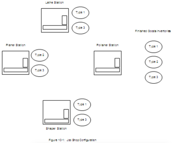
The job shop described in chapter 8 is being converted to a pull inventory control strategy as an intermediate step toward a full lean transformation. The shop consists of four workstations: lathe, planer, shaper, and polisher. The number of machines at each station was determined in chapter 8: 3 planers, 3 shapers, 2 lathes and 3 polishers. The time between demands for each item type is exponentially distributed. The mean time between demands for item type 1 is 2.0 hours, for type 2 items 2.0 hours, and for type 3 items 0.95 hours. The items have the following routes through the shop:

• Type 1: lathe, shaper, polisher
• Type 2: planer, polisher
• Type 3: planer, shaper, lathe, polisher

There is a supermarket following each workstation to hold the items produced by that station. Figure 10-1 shows the job shop configuration plus supermarkets, with job types in each supermarket identified. No routing information is shown. Improvements will be made at each station such that the processing times will be virtually constant and the same regardless of item type.

Planer:	1.533 hours
Shaper:	1.250 hours
Lathe:	0.8167 hours
Polisher:	0.9167 hours

Management anticipates changes in demand each month. The simulation model will be used as a tool to determine the number of kanbans to use in each month.

10.3.1 Define the Issues and Solution Objective

Management wishes to achieve a 99% service level provided to customers. The service level is defined as the percent of customer demands that can be statisfied from the finished goods inventories at the time the demand is made. At the same time, management wishes to minimize the amount of finished goods and in process inventory to control costs.

Thus initially, management wishes to determine the minimum number of kanbans for each item type associated with each inventory. The minimum number of kanbans establishes the maximum number of items of each type in each inventory.

10.3.2 Build Models

The process of the flow of control information through the job shop will be the perspective for model building. Note that the flow of control information from workstation to workstation follows the route for processing an item type in reverse order. For example, the route for type 1 items is lathe, shaper, polisher but the flow of control information is polisher, shaper, lathe.

The control information must include the name of the supermarket into which an item is placed upon completion at a workstation with the number of items of each type in the supermarket tracked. In addition, the control information should include the name of the inventory from which an item is taken for processing at a workstation. Supermarket / inventory names are constructed as follows. For the finished goods inventories, the name is INV_FINISHED_ItemType = INV_FINISHED_1 if ItemType = 1 and so forth. For the work in process inventories the name is INV_Station_ItemType, for example INV_SHAPER_1 for type one 1 items that have been completed by the shaper. Thus, the polisher places type 1 items in the inventory INV_FINISHED_1 and removes items from INV_SHAPER_1 since the shaper was the preceding station to the polisher on the production route of a type 1 item. Table 10-1 summarizes the supermarkets / inventories associated with each item type at each workstation. In the model, a distinct state variable models each of the inventories.

Table 10-1: Inventory Names by Item Type and Station

Supermarket / Inventory	Item Type	Output from Station	Input to Station or Customer
INV_FINISHED_1	1	Polisher	Customer
INV_FINISHED_2	2	Polisher	Customer
INV_FINISHED_3	3	Polisher	Customer
INV_SHAPER_1	1	Shaper	Polisher
INV_LATHE_1	1	Lathe	Shaper
INV_PLANER_2	2	Planer	Polisher
INV_LATHE_3	3	Lathe	Polisher
INV_SHAPER_3	3	Shaper	Lathe
INV_PLANER_3	3	Planer	Shaper

The transmission of control information via a kanban is initiated when a finished item is removed from an inventory. The station preceding the FGI, in this case the polisher for all item types, is instructed to complete an item to replace the one removed from the FGI. The polisher station removes a partially completed item from an inventory, for example INV_SHAPER_1 for item type 1, for processing. The item completed by the polisher is placed in the appropriate FGI. The removal of a partially completed item from INV_SHAPER_1 is followed immediately by processing at the shaper to complete a replacement item. This processing at the polisher and shaper can occur concurrently. Information flow and processing continues in this fashion until all inventories for the particular type of item have been replenished.

Each entity has the following attributes:
ArriveTime:	time of arrival of a demand for a job in inventory
JobType:	type of job
Location:	location of the production control information (kanban) relative to the start of the route of a job: 1..4
Routei:	station at the ith location on the route of a job
P_Invi:	the name of the inventory from which a partially completed item is removed for processing at the ith location on the route of a job
F_Invi:	the name of the inventory into which the item completed at the workstation is placed at the ith location on the route of a job

The arrival process for type one jobs is shown below. Arrivals represent a demand for a finished item that subsequent triggers the production process to replace the item removed from inventory to satisfy the demand.

The entity attributes are assigned values. Notice that the value of location is set initially to one greater than the ending position on the route. Thus, production is triggered at the last station on the route, which triggers production on the second last station on the route, and so forth.

The arrival process model includes removing an item from a FGI. Thus arriving entites wait for a finished item to be in inventory, remove an item when one is available, and update the number of finished items in the inventory.

---

Define Arrivals: \(\ \quad \quad\)Type1 \(\ \quad \quad\quad \quad\)Time of first arrival: \(\ \quad \quad\quad \quad\)Time between arrivals: \(\ \quad \quad\)Type2 \(\ \quad \quad\quad \quad\)Time of first arrival: \(\ \quad \quad\quad \quad\)Time between arrivals: \(\ \quad \quad\)Type3 \(\ \quad \quad\quad \quad\)Time of first arrival: \(\ \quad \quad\quad \quad\)Time between arrivals:	0 Exponentially distributed with a mean of 2 hours Number of arrivals: Infinite 0 Exponentially distributed with a mean of 2 hours Number of arrivals: Infinite 0 Exponentially distributed with a mean of 0.95 hours Number of arrivals: Infinite
Define Resources: \(\ \quad \quad\)Lathe/2 \(\ \quad \quad\)Planer/3 \(\ \quad \quad\)Polisher/3 \(\ \quad \quad\)Shaper/3	with states (Busy, Idle) with states (Busy, Idle) with states (Busy, Idle) with states (Busy, Idle)
Define Entity Attributes: \(\ \quad \quad\)ArrivalTime \(\ \quad \quad\)JobType \(\ \quad \quad\)Location \(\ \quad \quad\)Route(5) \(\ \quad \quad\)ArriveStation \(\ \quad \quad\)F_Inv(4) \(\ \quad \quad\)P_Inv(4)	// part tagged with its arrival time; each part has its own tag // type of job // location of a job relative to the start of its route: 1..4 // station at the ith location on the route of a job // time of arrival to a station, used in computing the waiting time // the name of the inventory into which a completed item is placed // at the ith location on the route // the name of the inventory from which an item to be completed // is taken at the ith location on the route
Process ArriveType1 Begin \(\ \quad \quad\)Set ArrivalTime = Clock \(\ \quad \quad\)Set JobType = 1 \(\ \quad \quad\)Set Location = 4 \(\ \quad \quad\)// Set route \(\ \quad \quad\)Set Route(1) to P_Lathe \(\ \quad \quad\)Set Route(2) to P_Shaper \(\ \quad \quad\)Set Route(3) to P_Polisher \(\ \quad \quad\)// Set following inventories \(\ \quad \quad\)Set F_Inv(1) to I1Lathe \(\ \quad \quad\)Set F_Inv(2) to I1Shaper \(\ \quad \quad\)Set F_Inv(3) to I1Final \(\ \quad \quad\)// Set preceding inventories \(\ \quad \quad\)Set P_Inv(1) to NULL \(\ \quad \quad\)Set P_Inv(2) to I1Lathe \(\ \quad \quad\)Set P_Inv(3) to I1Shaper \(\ \quad \quad\)// Get and update inventory \(\ \quad \quad\)Wait until I1Final > 0 \(\ \quad \quad\)Set I1Final -- \(\ \quad \quad\)// Record service level \(\ \quad \quad\)If (Clock > ArrivalTime) then \(\ \quad \quad\)Begin \(\ \quad \quad\)// Arrival waited for inventory \(\ \quad \quad\quad \quad\)tabulate 0 in ServiceLevel1 \(\ \quad \quad\quad \quad\)tabulate 0 in ServiceLevelAll \(\ \quad \quad\)End \(\ \quad \quad\)Else \(\ \quad \quad\)Begin \(\ \quad \quad\)// Arrival immediately acquired inventory \(\ \quad \quad\quad \quad\)tabulate 100 in ServiceLevel1 \(\ \quad \quad\quad \quad\)tabulate 100 in ServiceLevelAll \(\ \quad \quad\)End \(\ \quad \quad\)Send to P_Router End	// record time job arrives on tag // type of job // job at start of route // NULL is a constant indicating no inventory

---

The process at a station includes requesting and receiving items in inventory from preceding stations, processing a item, and placing completed items in inventory at the station. All stations follow this pattern but differ somewhat from each other.

As shown in Figure 10-1, no operations precede the planer station for any item type. Thus information triggering additional production at other stations is unnecessary. Upon completion of the planer operation, a job is added to the inventory whose name is the value of entity attribute F_INV[Location], for example INV_PLANER_1.

The process model of the shaper station is like the process model of the planer station with the retrieval of partially completed items from preceding workstations added. As soon as a partially completed item is retrieved, the routing process is invoked to begin generating the replacement for the item removed from inventory.

The lathe station model is similar to the shaper station model, except that it is the first station on the route for items of type 1. The polisher station model is similar to the shaper station model. Developing the process models of the lathe and polisher stations is left as an exercise for the reader. The shaper and planer station models are shown below.

---

Process Shaper
// Shaper Station
Begin
\(\ \quad \quad\)// Acquire Preceeding Inventory
\(\ \quad \quad\)Wait until P_Inv(Location) > 0 in Q_Shaper Set P_Inv(Location) --
\(\ \quad \quad\)Clone to P_Router

\(\ \quad \quad\)// Process item on Shaper
\(\ \quad \quad\)Wait until Shaper is Idle in Q_Shaper Make Shaper Busy
\(\ \quad \quad\)Wait for 1.25 hours
\(\ \quad \quad\)Make Shaper Idle
\(\ \quad \quad\)Set F_Inv(Location)++
End

Process Planer
//Planer Station
Begin
\(\ \quad \quad\)// Acquire Preceeding Inventory
\(\ \quad \quad\)If P_Inv(Location) != NULL) then
\(\ \quad \quad\)Begin
\(\ \quad \quad\quad \quad\)Wait until P_Inv(Location) > 0 in Q_Planer
\(\ \quad \quad\quad \quad\)P_Inv(Location) --
\(\ \quad \quad\quad \quad\)Clone to P_Router
\(\ \quad \quad\)End

\(\ \quad \quad\)// Process item on Planer
\(\ \quad \quad\)Wait until Planer is Idle in Q_Planer Make Planer Busy
\(\ \quad \quad\)Wait for 0.9167 hours
\(\ \quad \quad\)Make Planer Idle
\(\ \quad \quad\)Set F_Inv(Location)++
End

---

The routing process is shown below. The attribute Location is updated by subtracting one from the current value. If the control information has been processed by the first workstation on a route, Location is equal to zero and nothing else needs to be done. Otherwise, the control information is sent to the preceding workstation on the route.

---

Process Router
Begin
\(\ \quad \quad\)Location - -
\(\ \quad \quad\)If Location > 0 then send to Route(Location)
End

---

Note the evolution of the model presented in chapter 8 into the model presented in this chapter. The routing process has been modified to send control information through a series of workstations in the reverse order of item movement for processing. This is how the model of the push system orientation was modified to represent a pull system orientation.

Arrivals are interpreted as demands for an item from a finished goods inventory instead of a new item to process. Processing of a new item is triggered via the routing process when a demand is satisfied from the inventory.

Inventory management is added to the model for FGI's for each type of item as well as inventories of partially completed items.

10.3.3 Identify Root Causes and Assess Initial Alternatives

The design of the simulation experiment is summarized in Table 10-2. Management has indicated that demand is expected to change monthly. Thus, a terminating experiment with a time interval of one month is employed. There are three random number streams, one for the arrival process of each item type. Twenty replicates are made. Since stations are busy only in response to a demand, all stations idle is a reasonable state for the system and thus appropriate for initial conditions.

Table 10-2: Simulation Experiment Design for the Just-in-Time Job Shop
Element of the Experiment	Values for This Experiment
Type of Experiment	Terminating
Model Parameters and Their Values	Initial number of items of each type in each inventory 1. Infinite 2. Number needed to provide a 99% service level for the average time to replace an item in the finished goods inventory
Performance Measures	1. Number of items of each type in each buffer 2. Customer service level
Random Number Streams	Three, one for the arrival process of each item type.
Initial Conditions	Idle stations
Number of Replicates	20
Simulation End Time	184 hours (one month)

The experimental strategy is to determine a lower and an upper bound on the inventory level and thus the number of kanbans. First, the minimum inventory level needed for a 100% service level will be determined. This is the maximum inventory level that would ever be used that is the upper bound. The lower bound is the number of items in finished goods inventory needed to achieve a 99% service level for the average time to replace an item taken from the finished goods inventory. The service level in this case will likely be less than 99% since the time to replace some units will be greater than this average.

Prior information is information known before the simulation results are generated that is used along with these results to reach a conclusion. In this case, the following prior information is available.

1. For each item type, the number of kanbans associated with each inventory (finished goods and work in process at each station) should be the same by management policy.
2. All inventories for an item type should be the same as the finished goods inventory level.
3. The finished goods inventory level for a product relative to the other products should be proportional to the arrival rate of the demand for that product relative to the arrival rate of the demand for all products together, at least approximately.

The first piece of prior information makes the kanban control system simpler to operate since the number of kanbans depends only on the product, not the workstation as well. The second point recognizes that the service level depends on the availability of items in a finished goods inventory when a customer demand occurs. The service level does not depend on the availability of partially completed items in other inventories when requested by a workstation for further processing.

The third point recognizes that the number of kanbans should be balanced between products with respect to customer demand. Table 10-3 show the computations necessary to determine the percent of the customer demand that is for each product. The demand per hour is the reciprocal of the time between demands. The sum of the demand per hour for each item is the total demand per hour. Thus, the percent of the demand for each item is determined as the demand per hour for that item divided by the total.

Table 10-3: Percent of Demand from Each Product
Item	Time Between Demands	Demand per hour	% of Demand
1	2.00	0.50	24%
2	2.00	0.50	24%
3	0.95	1.05	52%
Total	0.49	2.05	100%

The upper bound on the number of kanbans associated with each inventory, equal to the number of items in each inventory in this case, is estimated as follows. The initial number of items in an inventory is set to infinite. In other words, the state variable modeling the inventory is initially set to a very large number. Thus, there will be no waiting for a needed item because it is not in inventory. The inventory level will be observed over time. The minimum inventory level observed in the simulation represents the number of units that were never used and thus are not needed.

Setting the inventory level as discussed in the previous paragraph implies that the service level would be 100% since by design there is always inventory to meet a customer demand.

The simulation results for the infinite inventory case are shown in Table 10-4. These results can be interpreted using the prior information discussed above. In this way, the number of kanbans in each inventory for each item is the same as the finished goods inventory for that item. Thus, the upper bound on the number of items need in each inventory is 4 for item type 1, 4 for item type 2 and 6 for item type 3. Thus, a total of 44 items are needed in inventory.

Note that the percent of the total finished goods inventory for each item is near the percent demand shown in Table 10-3: Type 1, 29% from the simulation versus 24% of the demand; Type 2, 29% versus 24% and Type 3, 44% versus 52%. Further, the percent of the total for type 1 and type 2 are equal to each other as in Table 10-3. Thus, validation evidence is obtained.

Table 10-4: Maximum Inventory Values from the Pull Job Shop Simulation
Replicate	FGI Type 1	Lathe Type 1	Shaper Type 1	FGI Type 2	Planer Type 2	FGI Type 3	Lathe Type 3	Planer Type 3	Shaper Type 3
1	4	3	4	4	4	7	6	5	7
2	4	5	4	4	3	5	5	5	6
3	4	4	5	5	5	9	9	9	10
4	3	4	4	4	4	5	6	5	7
5	4	4	4	4	4	4	4	4	5
6	3	3	4	6	6	5	5	5	6
7	4	4	5	3	3	6	6	5	6
8	5	4	5	4	4	6	6	5	7
9	4	4	4	4	4	5	6	5	6
10	4	4	4	4	4	6	6	6	7
11	3	3	3	4	4	5	5	5	7
12	3	3	4	5	5	12	13	11	14
13	3	3	4	4	4	6	5	5	6
14	3	3	4	4	4	4	5	4	5
15	4	3	4	4	4	7	7	5	7
16	3	3	4	4	4	5	5	5	6
17	3	3	4	4	4	5	5	5	6
18	5	5	6	4	4	5	4	5	6
19	4	4	4	4	4	6	6	6	7
20	3	4	4	4	4	7	6	6	7
Average	3.7	3.7	4.2	4.2	4.1	6.0	6.0	5.6	6.9
Std. Dev.	0.671	0.671	0.616	0.587	0.641	1.835	1.974	1.638	1.971
99% CI Lower Bound	3.2	3.2	3.8	3.8	3.7	4.8	4.7	4.5	5.6
99% CI Upper Bound	4.1	4.1	4.6	4.5	4.5	7.2	7.3	6.6	8.2
Proposed Initial Capacity	4	4	4	4	4	6	6	6	6
% of Total FGI	29%			29%		44%

Alternatively, the number of items in inventory, and hence the number of kanbans, will be estimated as the number required to provide a 99% service level for the average time needed to replace a product taken from inventory. In other words, for the average time interval from when a product is taken by a customer from finished goods inventory till it is replaced in the finished goods inventory by the production system, the customer service level should be at least 99%. See Askin and Goldberg (2002) for a discussion of this strategy.

The average time interval to replace a product is the sum of two terms: the amount of time waiting for the polisher and the polisher processing time. The former can be determined using the VUT equation and adjusted here for multiple machines (m=3) as shown in equation 10-1.

\begin{align}C T_{q} \approx V U T=\left(\frac{c_{a}^{2}+c_{c T}^{2}}{2}\right)\left(\frac{\mu^{\sqrt{2(m+1)}-1}}{(1-\mu) * m}\right) C T\tag{10-1}\end{align}

The V term will be 0.5. The processing time at the polisher is a constant yielding zero for the coefficient of variation. The time between demands is exponentially distributed and thus has a coefficient of variation of 1. The utilization of the polisher is the processing time (0.9167 hours) divided by the number of machines at the polisher station (3) times the total number of units demanded per hour as shown in Table 10-3. Thus, the utilization of the polisher is 91.3%.

Using these values in equation 10-1 yields 0.1747 hours for the average waiting time before processing at the polisher. The average processing time at the polisher is 0.9167 hours. Thus, the average time for the polisher to complete one item is 1.0913 hours.

The finished goods inventory needed for each product must make the following probability statement true:

P(demand in 1.0913 hours \(\ \leq\) finished good inventory level) \(\ \geq\) 99%.

Since the time between demands for units is exponentially distributed, the number of units demanded in any fixed period of time is poisson distributed with mean equal to the average number of units demand in 1.0913 hours. The mean is computed as 1.0913 hours times the average number of units demand per hour shown in Table 10-3.

Table 10-5 shows the number of items in finished goods inventory needed to achieve at least a 99% service level for 1.0913 hours.

Table 10-5: Finished Goods Inventory Levels for the Average Time to Replace a Unit
Item	Expected Demand in 1.0913 Hours	Inventory Level	Service Level	Percent of Total Inventory
1	0.55	3	99.8%	30%
2	0.55	3	99.8%	30%
3	1.15	4	99.4%	40%
Total		10		100%

Note that the percent of total inventory for each product corresponds reasonably well to that given in Table 10-2, given the small number of units in inventory. Thus, validation evidence is obtained.

The lower bound on the total number of units in inventory is 31 which is 13 units less than the upper bound of 44.

Simulation results shown in Table 10-6 show the service level for each product and overall obtained when the inventory levels shown in Table 10-5 are used.

Table 10-6: Service Level Simulation Results for Finished Goods Inventory Levels (3, 3, 4)
Replicate	Type 1	Type 2	Type 3	Overall
1	98.1	98.8	97.2	97.8
2	97.8	97.6	98.9	98.4
3	96.7	92.6	89.9	92.2
4	100.0	100.0	95.9	97.9
5	98.6	98.8	100.0	99.3
6	100.0	94.1	98.9	97.8
7	96.8	100.0	96.7	97.4
8	97.6	94.4	95.0	95.5
9	98.9	99.0	96.7	97.8
10	97.6	98.9	94.4	96.2
11	100.0	96.9	97.5	97.9
12	100.0	93.2	86.1	91.1
13	100.0	98.8	96.4	97.8
14	100.0	98.8	100.0	99.7
15	98.9	93.9	96.1	96.3
16	100.0	98.9	98.5	99.0
17	100.0	98.7	98.4	98.8
18	96.8	98.9	98.9	98.4
19	98.0	98.9	96.3	97.4
20	100.0	95.7	95.8	96.7
Average	98.8	97.3	96.4	97.2
Std. Dev.	1.26	2.41	3.32	2.17
99% CI Lower Bound	98.0	95.8	94.3	95.8
99% CI Upper Bound	99.6	98.9<	98.5	98.6

The service levels are all less than the required 99% through the approximate 99% confidence interval for the service level of type 1 items contains 99%. Note in addition that the range of service levels across the replicates is small.

10.3.4 Review and Extend Previous Work

Management was pleased with the above results. It was thought, however, that the service level obtained when using the upper bound inventory values should be determined by simulation and compared to the service level obtained when using the lower bound values. This was done and the results are shown in Table 10-7.

Table 10-7: Comparison of Service Level for Two Inventory Capacities
	Type 1			Type 2			Type 3			Overall
Replicate	(3,3,4)	(4,4,6)	difference	(3,3,4)	(4,4,6)	difference	(3,3,4)	(4,4,6)	difference	(3,3,4)	(4,4,6)	difference
1	98.1	100.0	1.9	98.8	100.0	1.2	97.2	99.5	2.4	97.8	99.8	2.0
2	97.8	100.0	2.2	97.6	100.0	2.4	98.9	100.0	1.1	98.4	100.0	1.6
3	96.7	100.0	3.3	92.6	96.7	4.1	89.9	93.8	3.8	92.2	96.0	3.8
4	100.0	100.0	0.0	100.0	100.0	0.0	95.9	100.0	4.1	97.9	100.0	2.1
5	98.6	100.0	1.4	98.8	100.0	1.2	100.0	100.0	0.0	99.3	100.0	0.7
6	100.0	100.0	0.0	94.1	98.0	3.9	98.9	100.0	1.1	97.8	99.5	1.6
7	96.8	100.0	3.2	100.0	100.0	0.0	96.7	100.0	3.3	97.4	100.0	2.6
8	97.6	98.8	1.2	94.4	100.0	5.6	95.0	100.0	5.0	95.5	99.7	4.3
9	98.9	100.0	1.1	99.0	100.0	1.0	96.7	100.0	3.3	97.8	100.0	2.2
10	97.6	100.0	2.4	98.9	100.0	1.1	94.4	100.0	5.6	96.2	100.0	3.8
11	100.0	100.0	0.0	96.9	100.0	3.1	97.5	100.0	2.5	97.9	100.0	2.1
12	100.0	100.0	0.0	93.2	99.0	5.8	86.1	90.6	4.5	91.1	94.9	3.8
13	100.0	100.0	0.0	98.8	100.0	1.3	96.4	100.0	3.6	97.8	100.0	2.2
14	100.0	100.0	0.0	98.8	100.0	1.2	100.0	100.0	0.0	99.7	100.0	0.3
15	98.9	100.0	1.1	93.9	100.0	6.1	96.1	99.5	3.4	96.3	99.7	3.4
16	100.0	100.0	0.0	98.9	100.0	1.1	98.5	100.0	1.5	99.0	100.0	1.0
17	100.0	100.0	0.0	98.7	100.0	1.3	98.4	100.0	1.6	98.8	100.0	1.2
18	96.8	97.9	1.1	98.9	100.0	1.1	98.9	100.0	1.1	98.4	99.5	1.1
19	98.0	100.0	2.0	98.9	100.0	1.1	96.3	100.0	3.7	97.4	100.0	2.6
20	100.0	100.0	0.0	95.7	100.0	4.3	95.8	99.5	3.7	96.7	99.7	3.0
Average	98.8	99.8	1.0	97.3	99.7	2.3	96.4	99.1	2.8	97.2	99.4	2.3
Std. Dev.	1.26	0.53	1.14	2.41	0.85	1.95	3.32	2.45	1.61	2.17	1.39	1.14
99% CI Lower Bound	98.0	99.5	0.3	95.8	99.1	1.1	94.3	97.6	1.7	95.8	98.5	1.5
99% CI Upper Bound	99.6	100.2	1.8	98.9	100.2	3.6	98.5	100.7	3.8	98.6	100.3	3.0

The following can be noted from Table 10-7.

1. For the upper bound inventory values, (4, 4, 6), the approximate 99% service level confidence intervals include 99%.
2. The approximate 99% confidence intervals of the difference in service level do not contain zero. Thus, it can be concluded with 99% confidence that the service level provided by the lower bound on inventory values is less than that provided by the upper bound inventory values.
3. The approximate 99% confidence intervals of the difference in service level are relatively narrow.

Based on these results, management decided that an acceptable service level would be achieved by using a target inventory of 4 units for jobs of type 1 and 2 as well as 6 units for jobs of type 3.

10.3.5 Implement the Selected Solution and Evaluate

The selected inventory levels were implemented and the results monitored.