14.3: The Case Study

Resource requirements in a logistics system include capital expenditures for transportation mechanisms such as trucks and operating costs such as personnel salaries. Minimizing capital and operating expenditures while providing the level of service demanded by customers is a fundamental issue.

14.3.1 Define the Issues and Solution Objective

A new logistics system is being designed to deliver truck loads of finished product over a large area from a main terminal supporting a manufacturing plant. The logistics system works in a similar way to the one shown in Figure 14-1. Truck loads are shipped seven days per week every day of the year. For the next year, the daily shipping volume is estimated as follows: a minimum of 20, a mode of 35 and a maximum of 65. Thus, the average daily shipping volume is 40 loads per day \(\ \left(=\frac{(20+35+65)}{3}\right)\). This means that there are 14600 loads shipped per year on the average.

A truck waits at the terminal until it is loaded. Loading time is uniformly distributed between 2 and 4 hours. A sufficient number of workers are available for loading. The truck will make all of its deliveries and then return to the terminal. The time from the terminal to the customer site, in either direction, is triangularly distributed with a minimum of 4 hours, a mode of 12 hours and a maximum of 30 hours. The time at the customer site is triangularly distributed with a minumum of 2 hours, a mode of 4 hours, and a maximum of 8 hours.

Upon its return to the terminal, the truck must be inspected by a worker. Inspection time is uniformly distributed between 1 and 2 hours. Approximately 90% of the trucks pass inspection or require only minor adjustments and are then ready for another load. The other 10% require significant maintenance that is performed by the same worker. Repair time is triangularly distributed with a minimum of 4 hours, a mode of 8 hours and a maximum of 12 hours. Workers are available 16 hours per day.

Management does not want to significantly constrain the number of loads delivered each year. At the same time the number of trucks and number of workers needs to be minimized for cost reasons. Management has determined that differences of more than 1% in the number of round trips completed are operationally significant. This difference can affect company profitability. Difference of less than 1%, even if statistically significant, are considered to be operationally unimportant.

The objective is to determine the number of trucks and workers required for the effective operation of the product delivery system. Effective operation requires minimizing costs without significantly reducing the number of loads delivered.

14.3.2 Build Models

The expected number of trucks and workers needed can be estimated using simple algebra. This is a lower bound on the actual number of trucks and workers needed Simulation is used to determine if additional trucks and workers are needed to meet the delivery criteria established by management.

The expected time for a truck to complete the delivery process and be ready to begin another delivery is shown in Table 14-1.

Table 14-1: Expected Time to Complete Delivery Process

	Expected Time (Hours)
Load Truck	3.0
Travel to Customer	15.3
At Customer	4.7
Travel to Terminal	15.3
Inspection	1.5
Repair	0.8
Total	40.6

There are approximately 8760 hours in a year. Thus, a truck could be expected to make 215 deliveries per year ( = 8760 / 40.6). Thus, the number of trucks required to make 14600 deliveries is 68 ( = 14600 / 215).

The expected number of workers needed can be determined in the same way. A worker is required for inspection and repair with an expected time of 2.3 hours per delivery. Thus, a single worker who works 16 hours per day could inspect and repair on the average of 2539 trucks per year. Thus, 6 workers on each shift ( = 14600 / 2539) are needed.

The model of the logistics system can be divided into the following processes.

1. Daily generation of loads.
2. Truck loading and round trip to the customer site.
3. Truck inspection and repair.
4. Worker shift changes.

The first process Daily Loads operates as follows. The number of loads per day is generated as a sample from a triangular distribution with the appropriate minimum, mode, and maximum: 20, 35, 65. While the daily number of loads is an integer, it is also sufficiently large to model as a continuous random variable.

In order to avoid "loosing" fractional loads, the fractional part of the sample for one day is added to the number of loads for the next day. For example, suppose the value for the number of loads is 30.6. Then, 30 loads are created today and 0.6 is added to the number of loads for the following day. Suppose the value for the number of loads on the following day is 40.7. Next, 0.6 is added. Thus, 41 loads are created and 0.3 is added to the number of loads for the next day.

In this process, the variable LoadsWaiting contains the quantity described above and the variable NLoads contains the integer portion of LoadsWaiting. NLoads loads are sent to the second process, RoundTrip, each day.

---

Define Arrivals: \(\ \quad \quad\)Time of first arrival: \(\ \quad \quad\)Time between arrivals: \(\ \quad \quad\)Number of arrivals:	0 1 day Infinite
Define Variables \(\ \quad \quad\)LoadsWaiting \(\ \quad \quad\)NLoads: Integer	// Number of loads to ship // Integer number of loads to ship
Process Daily Begin \(\ \quad \quad\)Set LoadsWaiting += Triag 20, 35, 65 \(\ \quad \quad\)Set NLoads = LoadsWaiting \(\ \quad \quad\)Set LoadsWaiting -= NLoads \(\ \quad \quad\)Clone NLoads to RoundTrip End

---

The process model for truck loading and load delivery, RoundTrip, consists of four time delays, one each for truck loading, movement to the customer site, time at the customer site, and return to the terminal. Then the truck goes to the inspection process. Preceding the time delays, each load acquires a truck.

Preceding truck acquisition, the model determines whether an additional unit of the truck resource should be created. If the number of truck resource units is less than a specified limit, contained in the variable MaxTrucks, and there are no free units of the truck resource, then a new unit is created. Thus, the load would not wait for a truck. Else, the load must wait for a truck to return from a delivery as well as being inspected and repaired.

---

Define Variables \(\ \quad \quad\)MaxTrucks	// Maximun number of trucks
Define Resources \(\ \quad \quad\)Truck	// Trucks
Process RoundTrip Begin \(\ \quad \quad\)If Truck/1 is Idle is FALSE then \(\ \quad \quad\)Begin \(\ \quad \quad\)// Add another truck if possible \(\ \quad \quad\quad \quad\)If Truck Units < MaxTruck then \(\ \quad \quad\quad \quad\quad \quad\)Increment Truck Units by 1 \(\ \quad \quad\)End \(\ \quad \quad\)Wait Until Truck/1 is Idle in QTruck \(\ \quad \quad\)Make Truck/1 Busy \(\ \quad \quad\)Wait for \(\ \quad \quad\)Wait for \(\ \quad \quad\)Wait for \(\ \quad \quad\)Wait for \(\ \quad \quad\)Send to Inspect End	uniform triangular triangular triangular	2, 4 hours 4, 12, 30 hours 2, 4, 8 hours 4, 12, 30 hours	//Loading Time //To Customer //At Customer //From Customer

---

Similar logic is used to model the worker resource in the truck inspection and repair process, Inspect. After an entity acquires the worker resource, there is time delay for inspection. Ten percent of the entities also require a time delay for repair.

---

Define Variables \(\ \quad \quad\)MaxWorkers	// Maximun number of workers
Define Resources \(\ \quad \quad\)Worker	// Inspection and repair workers
Process RoundTrip Begin \(\ \quad \quad\)If Worker/1 is Idle is FALSE then \(\ \quad \quad\)Begin \(\ \quad \quad\)// Add another worker if possible \(\ \quad \quad\quad \quad\)If Worker Units < MaxWorker then \(\ \quad \quad\quad \quad\quad \quad\)Increment Worker Units by 1 \(\ \quad \quad\)End \(\ \quad \quad\)Wait Until Worker/1 is Idle in QWorker \(\ \quad \quad\)Make Worker/1 Busy \(\ \quad \quad\)Wait for uniform 3, 1 hr \(\ \quad \quad\)If uniform 0, 1 < 10% then \(\ \quad \quad\quad \quad\)Wait for triangular 4, 8, 12 \(\ \quad \quad\)Make Worker/1 Idle \(\ \quad \quad\)Make Truck/1 Idle End	//Inspection //Repair

---

The worker shift process is as was discussed in chapter 2. All units of the worker resource are put into the off-shift state after 16 hours of work and returned to the idle state after 8 hours.

Notice that this results in an approximation in the model. If a worker is inspecting or repairing a truck at the beginning of the off shift period, the inspection or repair will continue until completed. This worker will again be available for work at the beginning of the on-shift period. Thus, the number of workers required could be underestimated.

14.3.3 Identify Root Causes and Assess Initial Alternatives

The experimental strategy to determine the number of trucks and workers is as follows. First the number of trucks will be determined. After the number of trucks is established, the number of workers will be determined for that number of trucks.

The minimum number of trucks is the expected number, 68, as determined in the previous section. The maximum number will be determined through simulation by not constraining the number of units of the truck resource used, that is requiring that no load ever waits for a truck. Various values of the number of trucks between the minimum and the maximum will be simulated.

The number of workers is not constrained so that no returning truck waits for a worker.

For each of these values, 20 replicates will be made and the average number of completed round trips over the replicates computed. A graph showing the average number of completed trips versus the number of trucks can be constructed. Thus, the number of trucks to use is determined.

The experimental design for determining the number of trucks is shown in Table 14-2.

A terminating experiment of duration 1 year (8760 hours), the planning period for the logistics system is used. There is one random number stream for each time delay modeled as a random variable as well as a random number stream for determining the daily number of loads. An additional random number stream is needed to model the random choice as to whether a truck passes inspection.

The primary system performance measure is the number of round trips completed. The utilization of trucks and workers are of interest. The experiment will begin with all trucks at the terminal waiting to make a trip.

Table 14-2: Simulation Experiment Design for Determining the Number of Trucks

Element of the Experiment	Values for This Experiment
Type of Experiment	Terminating
Model Parameters and Their Values	1. Number of trucks - Various values between the minimum needed and the maximum used.
Performance Measures	1. Number of round trips completed 2. Utilization of trucks 3. Utilization of workers
Random Number Streams	1. Number of pallets each day 2. Truck loading time 3. Travel time to customer 4. Time at customer site 5. Travel time from customer to terminal 6. Time to inspect returning truck 7. Decision: Did truck pass inspection? 8. Time to repair truck
Initial Conditions	Empty buffers and idle resources
Number of Replicates	20
Simulation End Time	1 year

First the simulation is run with 68 trucks and then with maximum number of trucks used as determined by the simulation to be 144 with an approximate 99% confidence interval of (141.3, 146.3).

The maximum number of trucks case results in an average of 662 more round trip completions per year. This is an increase of 4.8% over case where 68 trucks are used. Furthermore, this difference is statistically significant as seen by the approximate 99% confidence interval for the difference.

Thus, it can be concluded that more than 68 trucks are needed and that the number of trucks needed is between 68 and 144.

Table 14-3: Number of Round Trips – Average Trucks and Maximum Trucks

Replicate	Maximum Trucks	Average Trucks	Difference
1	14738	13863	875
2	14374	13850	524
3	14697	13839	858
4	14564	13800	764
5	14345	13853	492
6	14527	13823	704
7	14278	13804	474
8	14421	13877	544
9	14638	13825	813
10	14357	13854	503
11	14611	13858	753
12	14791	13828	963
13	14507	13755	752
14	14477	13754	723
15	14442	13872	570
16	14447	13868	579
17	14397	13810	587
18	14308	13839	469
19	14501	13820	681
20	14469	13860	609
Average	14494.5	13832.6	661.9
Std. Dev.	142.7	35.0	147.5
99% CI Lower Bound	14403.2	13810.2	567.5
99% CI Upper Bound	14585.7	13855.0	756.2

Furthermore simulation experiments are run with 68, 70, 75, ..., 140, and 144 trucks. Results are shown in the following graph, Figure 14-3.

Figure 14-3: Round Trips versus Number of Trucks

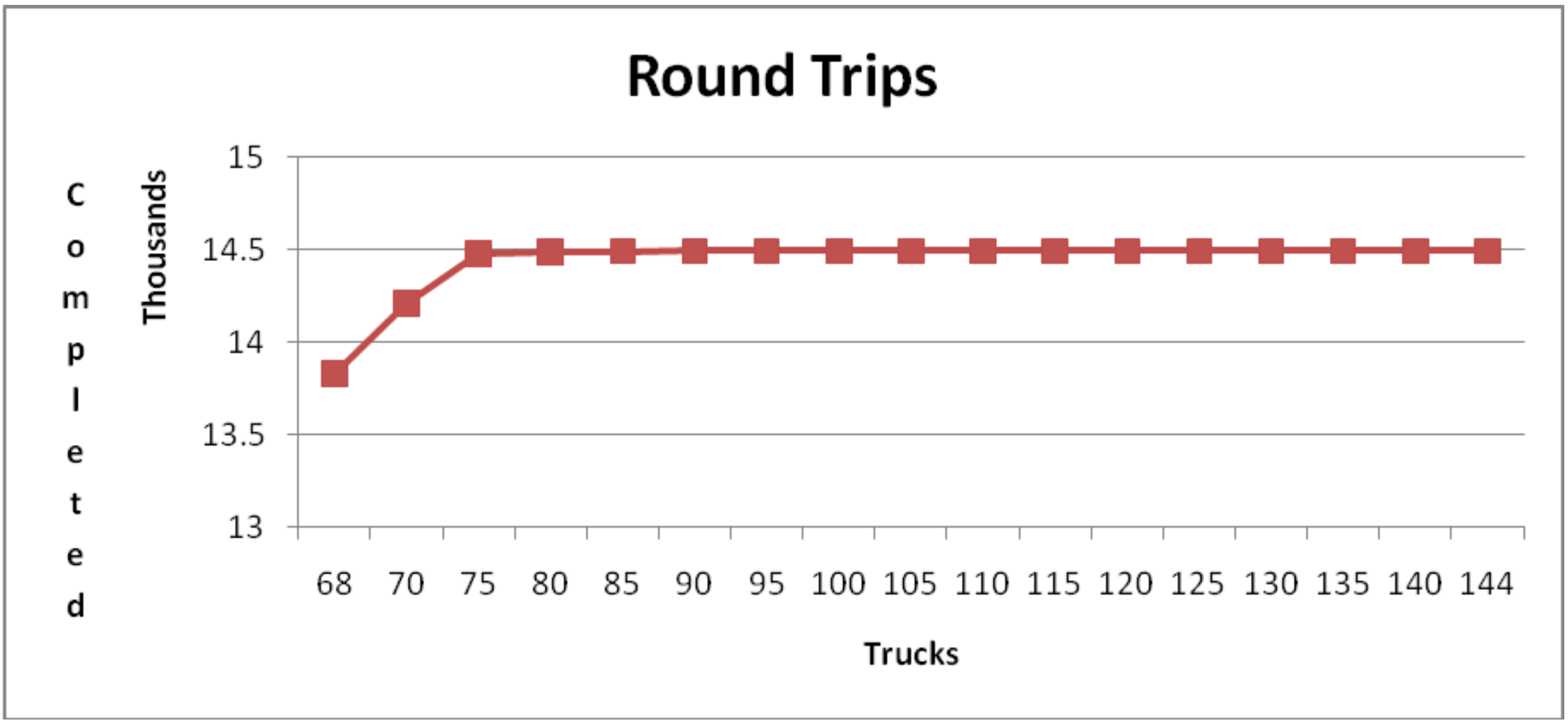
It appears from the graph that the number of roundtrips increases significantly up to 75 trucks. The difference in round trips when 80 trucks are used instead of 75 is only 14 on the average and thus is not operationally significant. Thus, 75 trucks will be used if there is a statistically and operationally significant difference in the number of roundtrips versus when 70 trucks are used. The simulation results are summarized in Table 14-4.

Table 14-4: Number of Round Trips – 75 Trucks versus 70 Trucks

Replicate	75 Trucks	70 Trucks	Difference (75 vs 70 Trucks)
1	14268	14715	447
2	14197	14351	154
3	14238	14669	431
4	14198	14558	360
5	14235	14341	106
6	14222	14527	305
7	14104	14273	169
8	14258	14385	127
9	14208	14601	393
10	14169	14320	151
11	14226	14604	378
12	14212	14704	492
13	14123	14497	374
14	14174	14477	303
15	14276	14433	157
16	14262	14439	177
17	14189	14397	208
18	14231	14307	76
19	14191	14486	295
20	14239	14435	196
Average	14211.0	14476.0	265.0
Std. Dev.	45.1	132.9	127.4
99% CI Lower Bound	14182.1	14390.9	183.5
99% CI Upper Bound	14239.9	14561.0	346.4

On the average, the number of roundtrips increases by 265, 1.9%, when 75 trucks are used versus 70 trucks. Thus, the difference is operationally significant since it is greater than 1%. The approximate 99% confidence interval for the difference is (183.5, 346.4). Thus, the difference is statistically significant.

Thus 75 trucks should be used. For this case, the truck utilization is 94.9% with an approximate 99% confidence interval of (94.1%, 95.3%). Utilization includes time spent in inspection and repair.

Given that 75 trucks should be used, the number of workers must be determined. The average maximum number of workers determined by the simulation experiments using 75 trucks is 30. This is the maximum number of workers that could be needed. The average number of workers computed with algebra was 6. The actual number of workers needed is somewhere between these two values. The simulation experiment to determine the number of workers is the same as that shown in Table 14-2 except that the model parameter is the number of workers instead of the number of trucks. Conducting this experiment is left as an exercise for the reader.

14.3.4 Review and Extend Previous Work

Management was pleased with the results as presented above and 75 trucks will be acquired.

14.3.5 Implement the Selected Solution and Evaluate

The number of completed roundtrips will be monitored. Additional trucks can be obtained and workers can be hired if needed.