
2.4: The Step Response
- Page ID
- 24395

Step Response
The impulse and step inputs are among prototype inputs used to characterize the response of the systems. The unit-step input is defined as:
\[ u(x)=\begin{cases}0, &\;x<0 \\ 1,&\; x\ge 0\end{cases} \nonumber \]
The step response of a system is defined as its response to a unit-step input, \(u(t)\), or \(u(s)=\frac{1}{s}\).
Let \(G(s)\) describe the system transfer function; then, the unit-step response is obtained as: \(y(s)\, \, =\, \, G(s)\frac{1}{s}\).
Its inverse Laplace transform leads to: \(y\left(t\right)={\mathcal{L}}^{-1}\left[\frac{G\left(s\right)}{s}\right]\).
Alternatively, the step response can be obtained by integrating the impulse response: \(y(t)=\int_0^t g(t-\tau)d\tau\).
The unit-step response of a stable system starts from some initial value: \(y\left(0\right)=y_0\), and settles at a steady-state value: \(y_{\infty }={\lim_{t\to \infty } y\left(t\right)\ }\).
Further, from the application of the final value theorem (FVT): \(y_{\infty }=G{\left(s\right)|}_{s=0}\).
Step Response of Low Order Systems
The unit-step response in the case of the first- and second-order systems is described below.
First-Order System
Let \(G(s)=\frac{K}{\tau s+1},\;\; u(s)=\frac{1}{s}\); then, \(y(s)=\frac{K}{s\left(\tau s+1\right)} =\frac{K}{s} -\frac{K\tau }{\tau s+1}\).
The time-domain response is given as: \(y(t)=K(1-e^{-t/\tau } )\, u(t)\).
Assuming arbitrary initial conditions, \(y\left(0\right)=y_0\), the step response of a first-order system is given as:
\[y\left(t\right)=y_{\infty }+\left(y_0-y_{\infty }\right)e^{-t/\tau },\ \ t\ge 0 \nonumber \]
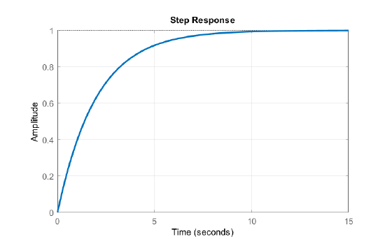
Let \(G(s)=\frac{1}{2s+1}\); then, the unit-step response is obtained as: \(y(s)=\frac{1}{s\left(2s+1\right)} =\frac{1}{s} -\frac{2}{2s+1}\).
The time-domain response is given as: \(y(t)=(1-e^{-t/2 } )\, u(t)\).
pkg load control
s=tf('s');
Gs=1/(2*s+1);
step(Gs), grid on

First-Order System with Integrator
Let \(G(s)=\frac{K}{s\left(\tau s+1\right)}, \;\;u(s)=\frac{1}{s}\); then, \(y(s)=\frac{K}{s^{2} \left(\tau s+1\right)}\).
Using PFE, we obtain: \(y(s)=K\left(\frac{1}{s^{2} } -\frac{\tau }{s} +\frac{\tau ^{2} }{\tau s+1} \right)\). Hence, \[g(t)=K\left(t-\tau \left(1-e^{-t/\tau } \right)\right)\, u(t) \nonumber \] The step response grows out of bound as \(t\to \infty\).
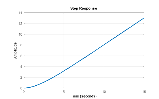
Let \(G(s)=\frac{1}{s(2s+1)}\); then, the unit-step response is computed as: \(y(s)=\frac{1}{s^2(2s+1)}=\frac{1}{s^2}-\frac{2}{s} +\frac{4}{2s+1}\).
The time-domain response is given as: \(y(t)=(t-2+2e^{-t/2 } )\, u(t)\).
pkg load control
s=tf('s');
Gs=1/s/(2*s+1);
step(Gs), grid on

Second-Order System with Real Poles
Let \(G(s)=\frac{K}{(\tau _{1} s+1)(\tau _{2} s+1)}\), \({\tau }_1>{\tau }_2\); then, the step response is computed as: \(y(s)=\frac{K}{s(\tau _{1} s+1)(\tau _{2} s+1)} =\frac{A}{s} +\frac{B}{\tau _{1} s+1} +\frac{C}{\tau _{2} s+1}\). Hence, \[y(t)=(A+Be^{-t/\tau _{1} } +Ce^{-t/\tau _{2} } )u(t) \nonumber \]
where \(A=K,B=-\frac{K{\tau }^2_1}{{\tau }_1-{\tau }_2},\ C=\frac{K{\tau }^2_2}{{\tau }_2-{\tau }_1}\).
A small DC motor has the following parameter values: \(R=1\; \Omega ,\; L=10\; {mH},\; J=0.01\; {kg-m}^{2} ,b=0.1\; \frac{N-s}{rad} ,\; k_{t} =k_{b} =0.05\).
The motor transfer function, from armature voltage to motor speed, is approximated as: \(G\left(s\right)=\frac{500}{\left(s+10\right)\left(s+100\right)}\).
The step response of the motor is obtained as: \(y\left(s\right)=\frac{1}{2s}-\frac{0.556}{s+10}+\frac{0.056}{s+100}\)
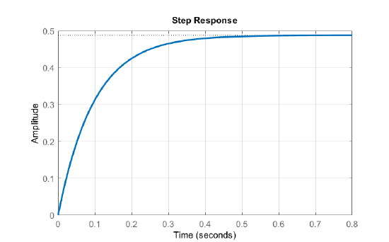
The time-domain response is given as: \(y\left(t\right)=\left(0.5-0.556e^{-10t}+0.056e^{-100t}\right)u(t)\), which settles at \(y_{\infty }=0.5\).
The natural response modes, \(e^{-10t}\) and \(e^{-100t}\), reflect motor electrical and mechanical time constants: \({\tau }_e\cong 0.01s\) and \( {\tau }_m\cong 0.1s\). The slower mechanical time constant dominates the motor step response.
pkg load control
s=tf('s');
Gs=500/(s+10)/(s+100);
step(Gs), grid on

Second-Order System with Complex Poles
Let \(G(s)=\frac{K}{(s+\sigma )^{2} +\omega _{d}^{2} }\). Then, the unit-step response is computed as: \(y(s)=\frac{A}{s} +\frac{Bs+C}{(s+\sigma )^{2} +\omega _{d}^{2} }\),
where \(A=G(0)=\frac{K}{\sigma ^{2} +\omega _{d}^{2} } ,\, \, B=-A,\, \, C=-2A\sigma\). Hence,
\[y(t)=\frac{K}{\sigma ^{2} +\omega _{d}^{2} } \left[1-e^{-\sigma t} \left(\cos \; \omega _{d} t+\frac{\sigma }{\omega _{d} } \sin \; \omega _{d} t\right)\right]u(t) \nonumber \]
In the phase form, the unit-step response is given as:
\[y(t)=\frac{K}{\sigma ^{2} +\omega _{d}^{2} } \left[1-e^{-\sigma t} \cos \; \left(\omega _{d} t-\phi \right)\right]\, u(t),\, \, \, \phi =\tan ^{-1} \frac{\sigma }{\omega _{d} } \nonumber \]
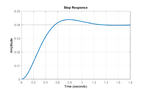
A mass–spring–damper system has the following parameter values: \(m=1\ kg,\ b=6\frac{Ns}{m},\ k=25\frac{N}{m}\).
Its transfer function is given as: \(G\left(s\right)=\frac{1}{s^2+5s+25}=\frac{1}{{\left(s+3\right)}^2+4^2}\). The system has complex poles located at: \(s=-3\pm j4\).
The unit-step response of the system is computed as: \(y\left(s\right)=\frac{1}{25}\left[\frac{1}{s}-\frac{s+6}{{\left(s+3\right)}^2+4^2}\right]\).
By applying the inverse Laplace transform, the time-domain response is obtained as:
\[y\left(t\right)=\frac{1}{25}\left[1-e^{-3t}\left({cos \left(4t\right)\ }+\frac{3}{4}{sin \left(4t\right)\ }\right)\right]u(t) \nonumber \]
pkg load control
s=tf('s');
Gs=1/(s^2+5*s+25);
step(Gs), grid on

System with Dead-time
The first-order-plus-dead-time (FOPDT) model of an industrial process is given as: \(G(s)=\frac{Ke^{-t_ds} }{\tau s+1}\), where \(\{K,\tau,t_d\}\) represent the process gain, time constant, and dead-time.
The step response of the FOPDT model is computed as: \(G(s)=\frac{Ke^{-t_ds} }{s(\tau s+1)}\), which translated into a time-domain response as: \(g(t)=(1-e^{-(t-t_d)/\tau})u(t-t_d)\).
An approximate process model, obtained by using Pade' approximation, is given as: \(G(s)=\frac{K(1-t_ds/2)}{(1+t_ds/2)(\tau s+1)}\). This model is termed as non-minimum phase due to the additional phase contributed by the right half-plane (RHP) zero.
The unit-step response of the approximate model is computed as: \(y(s)=\frac{K(1-t_ds/2)}{s(1+t_ds/2)(\tau s+1)}\).
The FOPDT model of a stirred-tank bio-reactor is given as: \(G(s)=\frac{20e^{-s} }{0.5s+1}\).
The step response of the system is computed as: \(y(s)=\frac{20e^{-s} }{s\left(0.5s+1\right)} \).
The time-domain response is obtained as: \(y(t)=20\left(1-e^{-2(t-1)} \right)\, u(t-1)\).
Using a first-order Pade’ approximation, an approximate process model is obtained as: \(G_{a} (s)=\frac{20\left(1-0.5s\right)}{\left(0.5s+1\right)^{2} }\).
The step response of the approximate model is computed as: \(y(s)=\frac{20\left(1-0.5s\right)}{s\left(0.5s+1\right)^{2} } \), \(y(t)=20\left(1-(1-4t)e^{-2t} \right)\, u(t)\).
The two responses are compared below (Figure 2.4.5). The step response for the FOPDT model starts after the designated delay. The step response for the Pade’ approximation starts with an undershoot due to the presence of RHP zero.
pkg load control
s=tf('s');
Gs=20/(.5*s+1);
t=0:.01:5;
u=ones(size(t));
u(1:100)=0;
lsim(Gs,u,t), grid on
hold
Gsa=20*(1-.5*s)/(1+.5*s)^2;
%step(Gsa)
lsim(Gsa,ones(size(t)),t,'r')
legend('sys with deadtime','pade approximation')

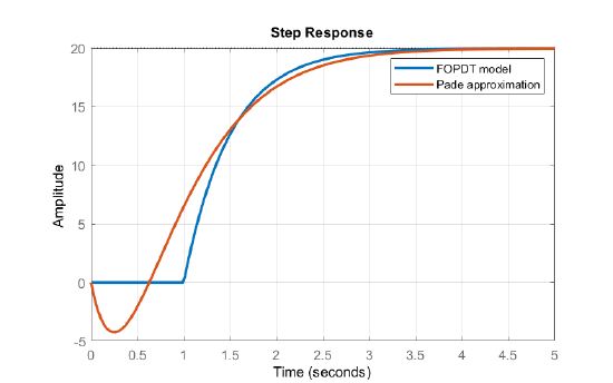
We make the following observations based on the figure:
- The step response of the process with dead-time starts after 1 s delay (as expected).
- The step response of Pade’ approximation of delay has an undershoot. This behavior is characteristic of transfer function models with zeros located in the right-half plane.