3.2: First-Order Dynamic Controllers

Dynamic Loop Controllers

A dynamic controller, \(K(s)\), in the feedback loop is a dynamic system that suitably conditions the error signal as \(u(s)=K(s)e(s)\) to affect the closed-loop system response. The feedback control system configuration is shown below where \(H(s)=1\) is assumed.

Figure \(\PageIndex{1}\): Feedback control system with plant, \(G(s)\), sensor, \(H(s)\), and controller, \(K(s)\).

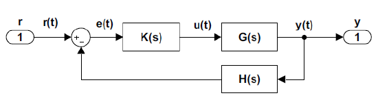
To analyze the feedback control system, assume that the plant is described by  \(G\left(s\right)=\frac{n\left(s\right)}{d\left(s\right)}\), and the dynamic controller is described by  \(K\left(s\right)=\frac{n_c\left(s\right)}{d_c\left(s\right)}\); then, the closed-loop transfer function from the reference input to the plant output is given as:

\[\frac{y\left(s\right)}{r\left(s\right)}=\frac{n\left(s\right)n_c\left(s\right)}{d\left(s\right)d_c\left(s\right)+n\left(s\right)n_c\left(s\right)}. \nonumber \]

The error transfer function from the reference input to the comparator output is given as:

\[\frac{e\left(s\right)}{r\left(s\right)}=\frac{1}{d\left(s\right)d_c\left(s\right)+n\left(s\right)n_c\left(s\right)}. \nonumber \]

The closed-loop characteristic polynomial is given as: \(\mathit{\Delta}\left(s\right)= d\left(s\right)d_c\left(s\right)+n\left(s\right)n_c\left(s\right)\).

First-Order Dynamic Controllers

In particular, we consider a first-order dynamic controller, described by the transfer function:

\[K\left(s\right)=K\left(\frac{s+z_c}{s+p_c}\right) \nonumber \]

The first-order controller adds a zero located at \(-z_c\) and a pole located at \(-p_c\) to the loop transfer function: \(KGH(s)\).

Let \(G(s)=\frac{n(s)}{d(s)}, \; H(s)=1\); then, the closed-loop characteristic polynomial with the controller in the loop is given as: \(\Delta(s)=d(s)(s+p_c)+n(s)(s+z_c)\).

Traditionally, first-order controllers are characterized as of phase-lead or phase-lag type, where lead and lag terms refer to the phase contribution from the controller to the Bode phase plot of the loop transfer function.

Let \(K\left(j\omega\right)=K\left(\frac{j\omega+z_c}{j\omega+p_c}\right)\); then, the phase angle contribution of the controller toward the loop transfer function is given as:

\[\angle K(j\omega )=\angle (j\omega+z_c)-\angle (j\omega+p_c)={\theta }_z-{\theta }_p \nonumber \]

where \({\theta }_z\) and \({\theta }_p\) denote the angles subtended by the controller pole and zero at a desired closed-loop pole location in the complex plane.

The phase contribution is positive for phase-lead controller and negative for phase-lag controller (see Figures 3.2.2 and 3.2.3 below).

Phase-Lead Controller

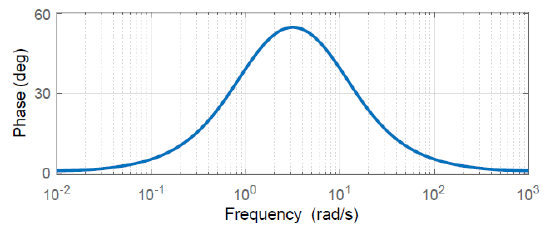
A phase-lead controller is characterized by \(z_{c} <p_{c}\), and contributes a net positive phase to the loop transfer function.

Example \(\PageIndex{1}\)

A phase-lead controller is expressed as: \(K\left(s\right)=\frac{s+1}{s+10}\). The phase contribution from the controller is shown below.

Figure \(\PageIndex{2}\): Phase contribution from a first-order phase-lead controller.

Phase-Lag Controller

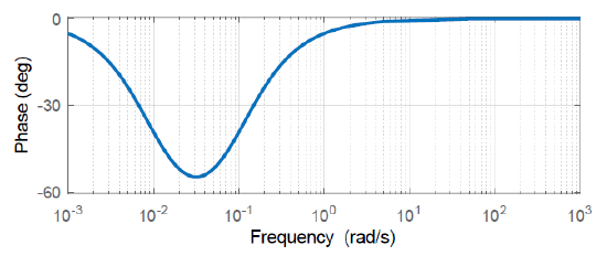
A phase-lag controller is characterized by \(z_{c} >p_{c}\), and contributes a net negative phase to the loop transfer function.

Example \(\PageIndex{2}\)

A phase-lead controller is expressed as: \(K\left(s\right)=\frac{s+0.1}{s+0.01}\). The phase contribution from the controller is shown below.

Figure \(\PageIndex{3}\): Phase contribution from a first-order phase-lag controller.

Lead-lag controller

A lead-lag controller is a second-order controller that combines a phase-lead section with a phase-lag section; it thus has the form:

\[K(s)=\frac{K(s+z_{1} )(s+z_{2} )}{(s+p_{1} )(s+p_{2} )} \nonumber \]

As an example, a lead-lag controller is given as: \(K(s)=\frac{K(s+0.1)(s+10)}{(s+1)^{2} } \).

We may note that the phase-lag zero is placed at a frequency much lower than the dominant pole frequency, whereas the phase-lead zero is placed in the vicinity of the dominant pole frequency.

Controller Design Example

The controller gain selection for a phase-lead design is explored in the following example.

Example \(\PageIndex{3}\)

The transfer function model for a position control system is given as: \(G\left(s\right)=\frac{1}{s\left(0.1s+1\right)}\).

Let a phase-lead controller for the model be defined by: \(K\left(s\right)=K\left(\frac{0.1s+1}{0.02s+1}\right)\).

Assuming \(H(s)=1\), the loop transfer function is formed as: \(KG\left(s\right)=\frac{K}{s\left(0.0.02s+1\right)}\).

The closed-loop characteristic polynomial is formulated as: \(\mathit{\Delta}\left(s,K\right)=s(0.02s+1)+K\).

Let a desired characteristic polynomial be given as: \({\mathit{\Delta}}_{des}\left(s\right)=0.02(s^2+50s+1000)\).

By comparing the coefficients, we obtain the controller gain as: \(K=20\).

Hence, the dynamic controller for the system is given as: \(K\left(s\right)=20\left(\frac{0.1s+1}{0.02s+1}\right)\).

We may note that when designing cascade controllers, not all closed-loop pole locations are reachable. The reachable pole locations can be found by the application of root locus technique (see Chapter 5).