3.1: Static Feedback Controller

Last updated
Save as PDF

Page ID: 24399

\( \newcommand{\vecs}[1]{\overset { \scriptstyle \rightharpoonup} {\mathbf{#1}} } \) \( \newcommand{\vecd}[1]{\overset{-\!-\!\rightharpoonup}{\vphantom{a}\smash {#1}}} \)\(\newcommand{\id}{\mathrm{id}}\) \( \newcommand{\Span}{\mathrm{span}}\) \( \newcommand{\kernel}{\mathrm{null}\,}\) \( \newcommand{\range}{\mathrm{range}\,}\) \( \newcommand{\RealPart}{\mathrm{Re}}\) \( \newcommand{\ImaginaryPart}{\mathrm{Im}}\) \( \newcommand{\Argument}{\mathrm{Arg}}\) \( \newcommand{\norm}[1]{\| #1 \|}\) \( \newcommand{\inner}[2]{\langle #1, #2 \rangle}\) \( \newcommand{\Span}{\mathrm{span}}\) \(\newcommand{\id}{\mathrm{id}}\) \( \newcommand{\Span}{\mathrm{span}}\) \( \newcommand{\kernel}{\mathrm{null}\,}\) \( \newcommand{\range}{\mathrm{range}\,}\) \( \newcommand{\RealPart}{\mathrm{Re}}\) \( \newcommand{\ImaginaryPart}{\mathrm{Im}}\) \( \newcommand{\Argument}{\mathrm{Arg}}\) \( \newcommand{\norm}[1]{\| #1 \|}\) \( \newcommand{\inner}[2]{\langle #1, #2 \rangle}\) \( \newcommand{\Span}{\mathrm{span}}\)\(\newcommand{\AA}{\unicode[.8,0]{x212B}}\)

Feedback Control System

The standard block diagram of a single-input single-output (SISO) feedback control system includes a plant, \(G(s)\), a controller, \(K(s)\), and a sensor, \(H(s)\), where \(H\left(s\right)=1\) is often assumed.

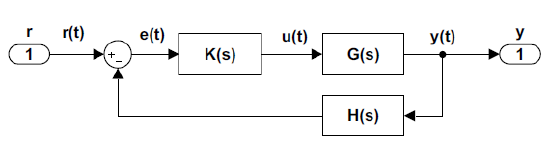
The overall system transfer function from input, \(r(t)\), to output, \(y(t)\), can be obtained by considering the error signal, \(e=r-Hy=r-KGHe\). Thus, \(\left(1+KGH\right)e=r\).

Let \(L\left(s\right)=KGH(s)\) denote the feedback loop gain; then, \(\left(1+L\right)e=r\).

The error transfer function from \(r\) to \(e\) is obtained as: \[S(s)=\frac{1}{1+L(s)}=\frac{1}{1+KGH(s)} \nonumber \]

The closed-loop transfer function from \(r\) to \(y\) is obtained as: \[T(s)=\frac{KG(s)}{1+KGH(s)} \nonumber \]

We may note that: \(S\left(s\right)+T\left(s\right)=1\).

Static Loop Controller Design

A static controller denotes the use of an amplifier with a gain, \(K\), to generate input to the plant, \(G(s)\). The controller action is represented as: \(u=Ke\), where \(e\) represents the error signal and \(u\) is the plant input.

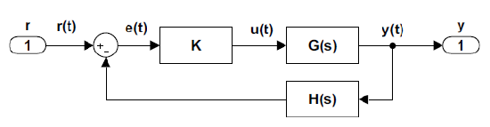
Figure \(\PageIndex{2}\): Feedback control system with static gain controller.

Assuming \(H(s)=1\), the closed-loop transfer function is given as:

\[\frac{y\left(s\right)}{r\left(s\right)}=T\left(s\right)=\frac{KG(s)}{1+KG\left(s\right)} \nonumber \]

Let \(G\left(s\right)=\frac{n\left(s\right)}{d\left(s\right)}\); then, the closed-loop transfer function is obtained as:

\[\frac{y\left(s\right)}{r\left(s\right)}=\frac{Kn\left(s\right)}{d\left(s\right)+Kn(s)} \nonumber \]

The closed-loop characteristic polynomial is defined as: \(\mathit{\Delta}\left(s,K\right)=d(s)+Kn\left(s\right)\).

From a controller design perspective, the gain \(K\) can be selected to achieve desirable root locations for the closed-loop characteristic polynomial. The design can be performed by comparing the coefficients of the characteristic polynomial with a desired characteristic polynomial.

Example \(\PageIndex{1}\)

The model for an environmental control system is given as: \(G\left(s\right)=\frac{1}{20s+1}\).

Assuming a static gain controller, the closed-loop characteristic polynomial is obtained as: \(\mathit{\Delta}\left(s,K\right)=20s+1+K\).

Suppose a desired characteristic polynomial is selected as: \({\mathit{\Delta}}_{des}\left(s\right)=4(5s+1)\). Then, by comparing the coefficients, we obtain the static controller as: \(K=3\).

Example \(\PageIndex{2}\)

Jun 22, 2020, 2:26 PM

Example 3.2:

The model for a position control system is given as: \(G\left(s\right)=\frac{1}{s\left(0.1s+1\right)}\).

Assuming a static gain controller, the characteristic polynomial is obtained as: \(\mathit{\Delta}\left(s,K\right)=s(0.1s+1)+K\).

Suppose a desired characteristic polynomial is selected as: \({\mathit{\Delta}}_{des}\left(s\right)=0.1(s^2+10s+50)\). Then, by comparing the coefficients, we obtain the static controller as: \(K=5\).