3.3: PI, PD, and PID Controllers
- Page ID
- 28514

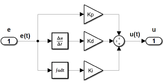
The PID Controller
The PID controller is a general-purpose controller that combines the three basic modes of control, i.e., the proportional (P), the derivative (D), and the integral (I) modes.
The PID controller in the time-domain is described by the relation:
\[u(t)=k_{p} +k_{d} \frac{d}{dt} e(t)+k_{i} \int e(t){d}t \nonumber \]
The PID controller has a transfer function:
\[K\left(s\right)=k_p+k_ds+\frac{k_i}{s} \nonumber \]
The controller gains for the three basic modes of control are given as: \(\left\{k_p,\ k_d,\ \ k_i\right\}\). Of these, the proportional term serves as a static controller, the derivative term helps speed up the system response, and the integral term helps reduce the steady-state error.
Closed-Loop Characteristic Polynomial
Let \(G(s)=\frac{n(s)}{d(s)}\); then the closed-loop characteristic polynomial with a PID controller in the loop is given as:
\[\Delta(s)=s\,d(s)+(k_ds^2+k_ps+k_i)\,n(s) \nonumber \]
For noise suppression, a first-order filter may be added to the PID controller; the modified controller transfer function is given as:
\[K(s)=k_{p} +\frac{k_{i} }{s} +\frac{k_{d} s}{T_{f} s+1} \nonumber \]
The filter additionally makes the controller transfer function proper and hence realizable by a combination of a low-pass and high-pass filters.
The control system design objectives may require using only a subset of the three basic controller modes. The two common choices, the proportional-derivative (PD) controller and the proportional-integral (PI) controller are described below.
PD Controller
A PD controller is described by the transfer function: \[K(s)=k_{p} +k_{d} s=k_{d} \left(s+\frac{k_{p} }{k_{d} } \right) \nonumber \]
A PD controller thus adds a single zero to the loop transfer function. The closed-loop characteristic polynomial is given as:
The phase contribution of the PD controller increases from \(0{}^\circ\) at low frequencies to \(90{}^\circ\) at high frequencies.
For practical reasons, a pole with a short time constant, \(T_f\), may be added to the PD controller. The pole helps limit the loop gain at high frequencies, which is desirable for disturbance rejection. The modified PD controller is described by the transfer function:
\[K(s)=k_p+\frac{k_ds}{T_fs+1} \nonumber \]
The modified PD controller is very similar to a first-order phase-lead controller; it is similarly employed to improve the transient response of the system.
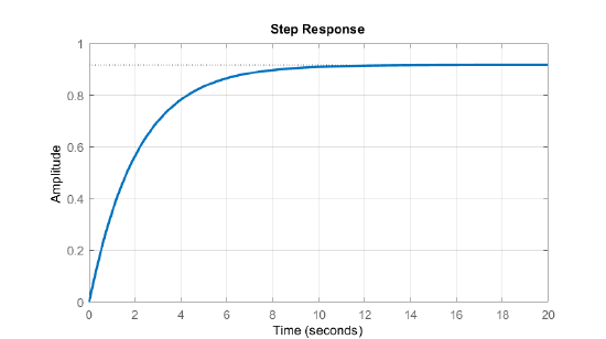
An environment control system is modeled as: \(G(s)=\frac{1}{25s+1}\). The model has a time constant of \(25\:sec\).
In order to speed up the response a PD controller with filter is designed as: \(K(s)=10+\frac{s}{.05s+1}\).
The closed-loop system has an effective time constant \(\tau\cong 2.5 \,sec\). The step response of the closed-loop system is plotted below.
PI Controller
A PI controller is described by the transfer function: \[K(s)=k_{p} +\frac{k_{i} }{s} =\frac{k_{p} (s+k_{i} /k_{p})}{s} \nonumber \]
The PI controller thus adds a pole at the origin (an integrator) and a finite zero to the feedback loop. The presence of the integrator in the loop forces the error to a constant input to go to zero in steady-state; hence PI controller is commonly used in designing servomechanisms.
The controller zero is normally placed close to the origin in the complex s-plane. The presence of a pole–zero pair adds a closed-loop system pole with a large time constant. The zero location can be adjusted so that the contribution of the slow mode to the overall system response stays small.
The PI-PD Controller
The PD and PI sections can be combined in a PI-PD controller as:
\[K(s)=\left(k_{p} +\frac{k_{i} }{s} \right)\left(1+k_{d} s\right)\;\; {\rm or} \;\; K(s)=\left(k_{p} +k_{d} s\right)\left(1+\frac{k_{i} }{s} \right) \nonumber \]
The PI-PD controller adds two zeros and an integrator pole to the loop transfer function. The zero from the PI part may be located close to the origin; the zero from the PD part is placed at a suitable location for desired transient response improvement.
The PI-PD controller is similar to a regular PID controller that is described by the transfer function:
\[K(s)=k_{p} +k_{d} s+\frac{k_{i} }{s} =\frac{k_{d} s^{2} +k_{p} s+k_{i} }{s} \nonumber \]
The PID controller imparts both transient and steady-state response improvements to the system. Further, it delivers stability as well as robustness to the closed-loop system.
PID Controller Tuning
The PID controller tuning refers to the selection of the controller gains: \(\; \left\{k_{p} ,\; k_{d} ,k_{i} \right\}\) to achieve desired performance objectives. Industrial PID controllers are often tuned using empirical rules, such as the Ziegler–Nicholas rules.
In the MATLAB Control System Toolbox, a PID controller object is created using the ‘pid’ command that can then be tuned with the ‘pidtune’ command. The MATLAB PID tuning algorithm aims for a \(60^{\circ }\) phase margin that results in a moderate \(10\%\) overshoot.
For a small DC motor, the following parameter values are assumed: \(R=1\, \Omega \; ,\; L=10\, {\rm mH},\; J=0.01\, kg\cdot m^{2} ,\; b=0.1\; \frac{N\cdot s}{rad} ,\; {\rm and}\, k_{t} =k_{b} =0.05\); the transfer function of the DC motor from armature voltage to motor speed is approximated as: \(G\left(s\right)=\frac{500}{\left(s+10\right)\left(s+100\right)}\).
The MATLAB tuned PID controller for the motor is given as:
\[K\left(s\right)=3.51+0.037s+\frac{56.2}{s} \nonumber \]
The MATLAB tuned PID controller with filter (PIDF) is given as:
\[K\left(s\right)=3.26+\frac{0.015s}{0.005s+1}+\frac{54.2}{s} \nonumber \]
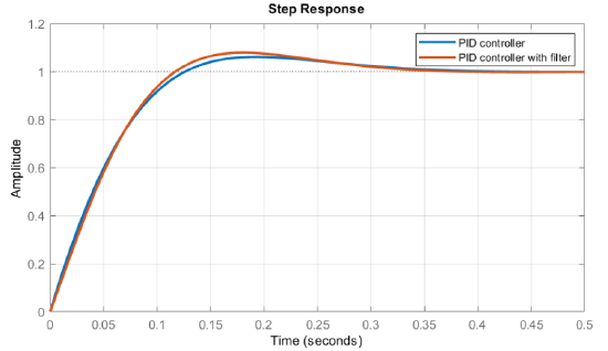
The response of the closed-loop system for the two controllers (PID and PIDF) is shown below (Figure 3.3.3). The response in both cases shows a settling time of 0.3sec with 7-8% overshoot and no steady-state error.