
3.4: Rate Feedback Controllers
- Page ID
- 28513

Rate Feedback Controllers
Rate feedback signal is often available from a tachometer or a rate gyro in position control applications. The signal can be employed to improve the response of the feedback control system.
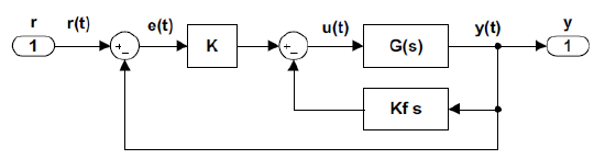
The basic rate feedback configuration (Figure 3.4.1) includes a rate constant \(k_f\) that multiplies the velocity signal together with a static controller, \(K\), in the loop.
The closed-loop transfer function for the rate feedback configuration can be obtained by applying Mason’s gain rule, originally defined for signal flow graphs. For simple block diagrams, the gain rule is stated as:
\[\frac{y\left(s\right)}{r\left(s\right)}=\frac{F(s)}{1-\sum L_i(s)} \nonumber \]
where \(F(s)\) denotes the forward path gain from an input node to an output node, and \(\sum L_i(s)\) denotes sum of the loop gains.
Rate Feedback as PD Controller
The effective loop gain in the case or rate feedback configuration with a static controller is computed as:
\[\sum L_i\left(s\right)=-G\left(s\right)\left(k_fs+K\right) \nonumber \]
The loop gain includes a plant transfer function in cascade with a PD controller, where the controller zero is located at: \(s=-\frac{K}{k_f}\). Hence rate feedback configuration is identical to placing a PD controller in the loop.
Let \(G\left(s\right)=\frac{n\left(s\right)}{d\left(s\right)};\) then, the closed-loop transfer function is obtained as:
\[\frac{y\left(s\right)}{r\left(s\right)}=\frac{Kn\left(s\right)}{d\left(s\right)+\left(k_fs+K\right)n\left(s\right)}, \nonumber \]
The resulting closed-loop characteristic polynomial is given as:
\[\mathit{\Delta}\left(s\right)=d\left(s\right)+\left(k_fs+K\right)n\left(s\right) \nonumber \]
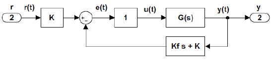
By using simple block diagram manipulation, the rate feedback configuration (Figure 3.4.1) can be equivalently represented as a feedback control system with a PD controller in the feedback path (Figure 3.4.2).
The transfer function of a mass–spring–damper system is given as: \(G\left(s\right)=\frac{1}{ms^2+bs+k}\). The following parameter values are assumed: \(m=1,b=2,\ and\ k=10\). It is desired to improve the transient response using rate feedback controller.
The closed-loop characteristic polynomial for the rate feedback configuration is:
\[\mathit{\Delta}\left(s\right)=s^2+\left(k_f+2\right)s+K+10 \nonumber \]
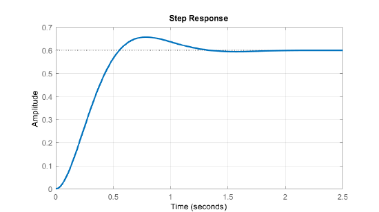
We assume that a desired characteristic polynomial is selected as: \({\mathit{\Delta}}_{des}\left(s\right)=\left(s^2+6s+25\right)\).
By comparing the polynomial coefficients, the required controller gains are obtained as: \(K=15,\ \ k_f=4\). The unit-step response of the closed-loop system is shown in Figure 3.4.3.
Rate Feedback as PID Controller
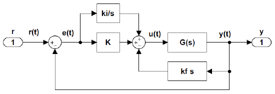
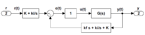
The rate feedback can be used in conjunction with a PI controller to effectively implement a PID controller. A rate feedback controller with cascade PID controller is shown in Figure 3.4.4.
Let the cascade PI controller be defined as: \(K_{PI}\left(s\right)=K+\frac{k_i}{s}\); then, using gain rule (3.4.1), the effective loop gain is obtained as:
\[\sum L_i\left(s\right)=-\left(K+\frac{k_i}{s}+k_fs\right)G\left(s\right) \nonumber \]
Hence using a cascade PI controller with rate feedback amounts to placing a PID controller in the feedback loop (Figure 3.4.5).
Assuming a plant transfer function: \(G\left(s\right)=\frac{n\left(s\right)}{d\left(s\right)},\) the closed-loop transfer function is obtained as:
\[\frac{y\left(s\right)}{r\left(s\right)}=\frac{\left(Ks+k_i\right)n\left(s\right)}{sd\left(s\right)+\left(k_fs^2+Ks+ki\right)n\left(s\right)}, \nonumber \]
The resulting closed-loop characteristic polynomial is given as:
\[\mathit{\Delta}\left(s\right)=sd\left(s\right)+\left(k_fs^2+Ks+k_i\right)n\left(s\right) \nonumber \]
The transfer function of a mass–spring–damper system is given as: \(G\left(s\right)=\frac{1}{ms^2+bs+k}\). The following parameter values are assumed: \(m=1,b=2,\ and\ k=10\). It is desired to improve the transient as well as steady-state response using rate feedback with cascade PI controller.
The closed-loop characteristic polynomial for the rate feedback configuration with cascade PI controller is given as:
\[\mathit{\Delta}\left(s\right)=s^3+\left(k_f+2\right)s^2+\left(K+10\right)s+k_i. \nonumber \]
We assume that a desired closed-loop characteristic polynomial is selected as: \({\mathit{\Delta}}_{des}\left(s\right)=\left(s^2+10s+25\right)\left(s+5\right)\).
Then, by comparing the polynomial coefficients, the controller gains are obtained as: \(k_f=13,\ \ K=65,\ \ and\ k_i=125\). The unit-step response of the closed-loop system is shown in Figure 3.4.6.
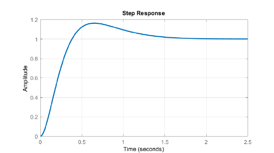
By comparing the step responses in Examples 3.4.1 and 3.4.2, we observe that:
- The rate feedback with cascade PI controller has a higher (\(18\%\)) overshoot compared to rate feedback with static controller (\(12\%\)).
- The rate feedback with cascade PI controller has a smaller rise time (\(0.3\,sec\)) compared to rate feedback with static controller (about \(0.5\,sec\)).
- The rate feedback with cascade PI controller has no steady-state error compared to (\(40\%\)) error in the case of rate feedback with static controller.
- The step response in both cases settles in about \(1.5\,sec\).