1.3: Tree Representations

Our estimates for the volume of a dollar bill (Section 1.1) and for the rail and highway capacities (Section 1.2) used the same method: dividing hard problems into smaller ones. However, the structure of the analysis is buried within the sentences, paragraphs, and pages. The sequential presentation hides the structure. Because the structure is hierarchical—big problems split, or branch, into smaller problems—its most compact representation is a tree. A tree representation shows us the analysis in one glance.

Here is the tree representation for the capacity of a train line. Unlike the biological variety, our trees stand on their head. Their roots, the goals, sit at the top of the tree. Their leaves, the small problems into which we have subdivided the goal, sit at the bottom. The orientation matches the way that we divide and conquer, filling the page downward as we subdivide.

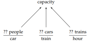
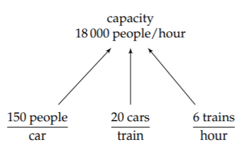
In making this first tree, we haven’t estimated the quantities themselves. We have only identified the quantities. The question marks remind us of our next step: to include estimates for the three leaves. These estimates were 150 people per car, 20 cars per train, and 6 trains per hour (giving the tree in the margin).

Then we multiplied the leaf values to propagate the estimates upward from the leaves toward the root. The result was 18 000 people per hour. The completed tree shows us the entire estimate in one glance.

This train-capacity tree had the simplest possible structure with only two layers (the root layer and, as the second layer, the three leaves). The next level of complexity is a three-layer tree, which will represent our estimate for the volume of a dollar bill. It started as a two-layer tree with three leaves.

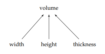
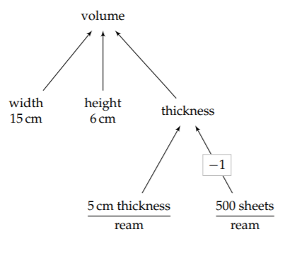
Then it grew, because, unlike the width and height, the thickness was difficult to estimate just by looking at a dollar bill. Therefore, we divided that leaf into two easier leaves.

The result is the tree in the margin. The thickness leaf, which is the thickness per sheet, has split into (1) the thickness per ream and (2) the number of sheets per ream. The boxed −1 on the line connecting the thickness to the number of sheets per ream is a new and useful notation. The −1 tells us the exponent to apply to that leaf value when we propagate it upward to the root.

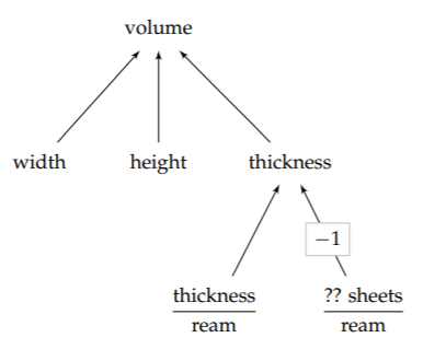
Here is why I write the −1 as a full-sized number rather than a small superscript. Most of our estimates require multiplying several factors. The only question for each factor is, “With what exponent does this factor enter?” The number −1 directly answers this “What exponent?” question. (To avoid cluttering the tree, we don’t indicate the most-frequent exponent of 1.)

This new subtree then represents the following equation for the thickness of one sheet:

\[thickness = \frac{thickness}{ream} \times (\frac{?? sheets}{ream})^{-1}\]

The −1 exponent allows, at the cost of a slight complication in the tree notation, the leaf to represent the number of sheets per ream rather than a less-familiar fraction, the number of reams per sheet.

Now we include our estimates for the leaf values. The width is 15 centimeters. The height is 6 centimeters. The thickness of a ream of paper is 5 centimeters. And a ream contains 500 sheets of paper. The result is the following tree.

Now we propagate the values to the root. The two bottommost leaves combine to tell us that the thickness of one sheet is 10⁻² centimeters. This thickness completes the tree’s second layer. In the second layer, the three nodes tell us that the volume of a dollar bill—the root—is 1 cubic centimeter

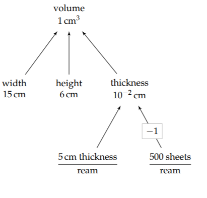
With practice, you can read in this final tree all the steps of the analysis. The three nodes in the second layer show how the difficult volume estimate was subdivided into three easier estimates. That the width and height remained leaves indicates that these two estimates felt reliable enough. In contrast, the two branches sprouting from the thickness indicate that the thickness was still hard to estimate, so we divided that estimate into two more-familiar quantities.

The tree encapsulates many paragraphs of analysis in a compact form, one that our minds can absorb in a single glance. Organizing complexity helps us build insight.

Exercise \(\PageIndex{1}\): Tree for the suitcase of bills

Make a tree diagram for your estimate in Problem 1.3. Do it in three steps: (1) Draw the tree without any leaf estimates, (2) estimate the leaf values, and (3) propagate the leaf values upward to the root.