9.5: Summary and further problems
- Page ID
- 24139
\( \newcommand{\vecs}[1]{\overset { \scriptstyle \rightharpoonup} {\mathbf{#1}} } \)
\( \newcommand{\vecd}[1]{\overset{-\!-\!\rightharpoonup}{\vphantom{a}\smash {#1}}} \)
\( \newcommand{\dsum}{\displaystyle\sum\limits} \)
\( \newcommand{\dint}{\displaystyle\int\limits} \)
\( \newcommand{\dlim}{\displaystyle\lim\limits} \)
\( \newcommand{\id}{\mathrm{id}}\) \( \newcommand{\Span}{\mathrm{span}}\)
( \newcommand{\kernel}{\mathrm{null}\,}\) \( \newcommand{\range}{\mathrm{range}\,}\)
\( \newcommand{\RealPart}{\mathrm{Re}}\) \( \newcommand{\ImaginaryPart}{\mathrm{Im}}\)
\( \newcommand{\Argument}{\mathrm{Arg}}\) \( \newcommand{\norm}[1]{\| #1 \|}\)
\( \newcommand{\inner}[2]{\langle #1, #2 \rangle}\)
\( \newcommand{\Span}{\mathrm{span}}\)
\( \newcommand{\id}{\mathrm{id}}\)
\( \newcommand{\Span}{\mathrm{span}}\)
\( \newcommand{\kernel}{\mathrm{null}\,}\)
\( \newcommand{\range}{\mathrm{range}\,}\)
\( \newcommand{\RealPart}{\mathrm{Re}}\)
\( \newcommand{\ImaginaryPart}{\mathrm{Im}}\)
\( \newcommand{\Argument}{\mathrm{Arg}}\)
\( \newcommand{\norm}[1]{\| #1 \|}\)
\( \newcommand{\inner}[2]{\langle #1, #2 \rangle}\)
\( \newcommand{\Span}{\mathrm{span}}\) \( \newcommand{\AA}{\unicode[.8,0]{x212B}}\)
\( \newcommand{\vectorA}[1]{\vec{#1}} % arrow\)
\( \newcommand{\vectorAt}[1]{\vec{\text{#1}}} % arrow\)
\( \newcommand{\vectorB}[1]{\overset { \scriptstyle \rightharpoonup} {\mathbf{#1}} } \)
\( \newcommand{\vectorC}[1]{\textbf{#1}} \)
\( \newcommand{\vectorD}[1]{\overrightarrow{#1}} \)
\( \newcommand{\vectorDt}[1]{\overrightarrow{\text{#1}}} \)
\( \newcommand{\vectE}[1]{\overset{-\!-\!\rightharpoonup}{\vphantom{a}\smash{\mathbf {#1}}}} \)
\( \newcommand{\vecs}[1]{\overset { \scriptstyle \rightharpoonup} {\mathbf{#1}} } \)
\(\newcommand{\longvect}{\overrightarrow}\)
\( \newcommand{\vecd}[1]{\overset{-\!-\!\rightharpoonup}{\vphantom{a}\smash {#1}}} \)
\(\newcommand{\avec}{\mathbf a}\) \(\newcommand{\bvec}{\mathbf b}\) \(\newcommand{\cvec}{\mathbf c}\) \(\newcommand{\dvec}{\mathbf d}\) \(\newcommand{\dtil}{\widetilde{\mathbf d}}\) \(\newcommand{\evec}{\mathbf e}\) \(\newcommand{\fvec}{\mathbf f}\) \(\newcommand{\nvec}{\mathbf n}\) \(\newcommand{\pvec}{\mathbf p}\) \(\newcommand{\qvec}{\mathbf q}\) \(\newcommand{\svec}{\mathbf s}\) \(\newcommand{\tvec}{\mathbf t}\) \(\newcommand{\uvec}{\mathbf u}\) \(\newcommand{\vvec}{\mathbf v}\) \(\newcommand{\wvec}{\mathbf w}\) \(\newcommand{\xvec}{\mathbf x}\) \(\newcommand{\yvec}{\mathbf y}\) \(\newcommand{\zvec}{\mathbf z}\) \(\newcommand{\rvec}{\mathbf r}\) \(\newcommand{\mvec}{\mathbf m}\) \(\newcommand{\zerovec}{\mathbf 0}\) \(\newcommand{\onevec}{\mathbf 1}\) \(\newcommand{\real}{\mathbb R}\) \(\newcommand{\twovec}[2]{\left[\begin{array}{r}#1 \\ #2 \end{array}\right]}\) \(\newcommand{\ctwovec}[2]{\left[\begin{array}{c}#1 \\ #2 \end{array}\right]}\) \(\newcommand{\threevec}[3]{\left[\begin{array}{r}#1 \\ #2 \\ #3 \end{array}\right]}\) \(\newcommand{\cthreevec}[3]{\left[\begin{array}{c}#1 \\ #2 \\ #3 \end{array}\right]}\) \(\newcommand{\fourvec}[4]{\left[\begin{array}{r}#1 \\ #2 \\ #3 \\ #4 \end{array}\right]}\) \(\newcommand{\cfourvec}[4]{\left[\begin{array}{c}#1 \\ #2 \\ #3 \\ #4 \end{array}\right]}\) \(\newcommand{\fivevec}[5]{\left[\begin{array}{r}#1 \\ #2 \\ #3 \\ #4 \\ #5 \\ \end{array}\right]}\) \(\newcommand{\cfivevec}[5]{\left[\begin{array}{c}#1 \\ #2 \\ #3 \\ #4 \\ #5 \\ \end{array}\right]}\) \(\newcommand{\mattwo}[4]{\left[\begin{array}{rr}#1 \amp #2 \\ #3 \amp #4 \\ \end{array}\right]}\) \(\newcommand{\laspan}[1]{\text{Span}\{#1\}}\) \(\newcommand{\bcal}{\cal B}\) \(\newcommand{\ccal}{\cal C}\) \(\newcommand{\scal}{\cal S}\) \(\newcommand{\wcal}{\cal W}\) \(\newcommand{\ecal}{\cal E}\) \(\newcommand{\coords}[2]{\left\{#1\right\}_{#2}}\) \(\newcommand{\gray}[1]{\color{gray}{#1}}\) \(\newcommand{\lgray}[1]{\color{lightgray}{#1}}\) \(\newcommand{\rank}{\operatorname{rank}}\) \(\newcommand{\row}{\text{Row}}\) \(\newcommand{\col}{\text{Col}}\) \(\renewcommand{\row}{\text{Row}}\) \(\newcommand{\nul}{\text{Nul}}\) \(\newcommand{\var}{\text{Var}}\) \(\newcommand{\corr}{\text{corr}}\) \(\newcommand{\len}[1]{\left|#1\right|}\) \(\newcommand{\bbar}{\overline{\bvec}}\) \(\newcommand{\bhat}{\widehat{\bvec}}\) \(\newcommand{\bperp}{\bvec^\perp}\) \(\newcommand{\xhat}{\widehat{\xvec}}\) \(\newcommand{\vhat}{\widehat{\vvec}}\) \(\newcommand{\uhat}{\widehat{\uvec}}\) \(\newcommand{\what}{\widehat{\wvec}}\) \(\newcommand{\Sighat}{\widehat{\Sigma}}\) \(\newcommand{\lt}{<}\) \(\newcommand{\gt}{>}\) \(\newcommand{\amp}{&}\) \(\definecolor{fillinmathshade}{gray}{0.9}\)Many physical processes contain a minimum-energy state where small deviations from the minimum require an energy proportional to the square of the deviation. This behavior is the essential characteristic of a spring. A spring is therefore not only a physical object but a transferable abstraction. This abstraction has helped us understand chemical bonds, sound speeds, and acoustic, electromagnetic, and gravitational radiation—and from there the colors of the sky and sunset.
Exercise \(\PageIndex{1}\): Two-dimensional acoustic
An acoustic line source is an infinitely long tube that can expand and contract. In terms of the source strength per length, find the power radiated per length.
Exercise \(\PageIndex{2}\): Decay of a lightly damped oscillation
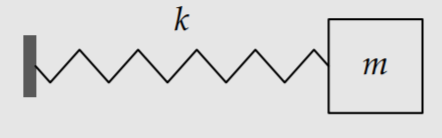
In an undamped spring–mass system, the motion is described by \(x = x_{0} \textrm{cos} \omega_{0} t\), where x0 is the amplitude and \(\omega_{0}\), the natural frequency, is k/m . In this problem, you use easy cases and lumping to find the effect of a small amount of (linear) damping. The damping force will be \(F = - \gamma v\), where \(\gamma\) is the damping coefficient and \(v\) is the velocity of the mass.
a. In terms of \(\omega_{0}\) and x0, estimate the typical speed and damping force, and then the typical energy lost to damping in 1 radian of oscillation (a time \(1/\omegea_{0}\)).
b. Express the dimensionless measure of energy loss
\[\frac{\Delta E}{E} = \frac{\textrm{energy lost per radian of oscillation}}{\textrm{oscillation energy}}\]
by finding the scaling exponent n in
\[\frac{\Delta E}{E} \sim Q^{n}\]
where Q is the quality factor from Problem 5.53. In terms of Q, what does “a small amount of damping” mean?
c. Find the rate constant C, built from Q and \(\omega_{0}\), in the time-averaged oscillation energy:
\[E \approx E_{0}e^{Ct},\]
d. Using the scaling between amplitude and energy, represent how the mass’s position x varies with time by finding the rate constant C′ in the formula
\[x(t) \approx x_{0} \textrm{cos} \omega_{0} t \times e^{C't},\]
Sketch x(t).
Exercise \(\PageIndex{3}\): Driving a spring at high frequency
Sunlight driving an electron in nitrogen is the easy-case regime \(\omega << \omega_{0}\). The opposite regime is \(\omega >> \omega_{0}\). This regime includes metals, where the electrons are free (the spring constant is zero, so \(\omega_{0}\) is zero). Estimate, using characteristic or typical values, the amplitude x0 of a spring–mass system driven by a force
\[F = F_{0} \textrm{cos} \omega t,\]
where \(\omega >> \omega_{0}\). In particular, find the scaling exponent n in the transfer function \(x_{0}/F_{0} \propto \omega^{n}\).
Exercise \(\PageIndex{4}\): High-frequency scattering
Use the result of Problem 9.12 to show that, in the \(\omega >> \omega_{0}\) regime (for example, for a free electron), the scattering cross section \(P_{\textrm{dipole}}/F\) is independent of \(\omega\) and is the Thomson cross section \(\sigma_{T}\).
Exercise \(\PageIndex{5}\): Fiber-optic cable
A fiber-optic cable, used fortransmitting telephone calls and other digital data, is a thin glass fiberthat carries electromagnetic radiation. High data transmission rates require a high radiation frequency \(\omega\). However, scattering losses are proportional to \(\omega^{4}\), so high-frequency signals attenuate in a short distance. As a compromise, glass fibers carry “near-infrared” radiation (roughly 1-micrometer in wavelength). Estimate the mean free path of this radiation by comparing the density of glass to the density of air.
Exercise \(\PageIndex{6}\): Resonance
In Problem \(\PageIndex{3}\), you analyzed the case of driving a spring at a frequency \(\omega\) much higher than its natural frequency \(\omega_{0}\). The discussion of blue skies in Section 9.4.1 required the opposite regime, \(\omega << \omega_{0}\). In this problem, you analyze the middle regime, which is called resonance. It is a lightly damped spring–mass system driven at its natural frequency.
Assuming a driving force \(F_{0} \textrm{cos} \omega t\), estimate the energy input per radian of oscillation, in terms of F0 and the amplitude x0. Using Problem 9.11(b), estimate the energy lost per radian in terms of the amplitude x0, the natural frequency \(\omega_{0}\), the quality factor Q, and the mass m.
By equating the energy loss and the energy input, which is the condition for a steady amplitude, find the quotient \(x_{0}/F_{0}\). This quotient is the gain G of the system at the resonance frequency \(\omega = \omega_{0}\). Find the scaling exponent n in \(G \propto Q_{n}\).
Exercise \(\PageIndex{7}\): Ball resting on the ground as a spring system
A ball resting on the ground can be thought of as a spring system. The larger the compression \(\delta\), the larger the restoring force F. Imagine setting weights on top of the ball so that the extra weight plus the ball’s weight is F.) Find the scaling exponent n in \(F \propto \delta^{n}\). Is this system an ideal spring (for which n = 1)?
Exercise \(\PageIndex{8}\): Inharmonicity of piano strings
An ideal piano string is under tension and has vibration frequencies given by
\[f_{n} = \frac{n}{2L} \sqrt{\frac{T}{\rho A}},\]
where A is its cross-sectional area, T is the tension, L is the string length, and n = 1, 2, 3, …. (In Section 9.2.2, we estimated \(f_{1}\).) Assume that the string’s cross section is a square of side length b. The piano sounds pleasant when harmonics match: for example, when the second harmonic (\(f_{2}\)) of the middle C string has the same frequency as the fundamental (\(f_{1}\)) of the C string one octave higher.
However, the stiffness of the string (its resistance to bending) alters these frequencies slightly. Estimate the dimensionless ratio
\[\frac{\textrm{potential energy from stiffness}}{\textrm{potential energy from stretching (tension)}}.\]
This ratio is also roughly the fractional change in frequency due to stiffness. Write this ratio in terms of the mode number n, the string side length (or diameter) b, the string length L, and the tension-induced strain \(\epsilon\).
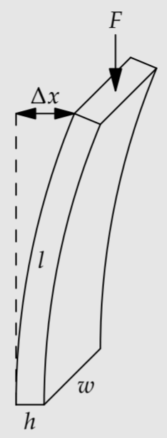
Exercise \(\PageIndex{9}\): Buckling
In this problem you estimate the force required to buckle a strut, such as a leg bone landing on the ground. The strut has Young’s modulus Y, thickness h, width w, and length l. The force F has deflected the strut by \(\Delta x\), producing a torque \(F \Delta x\). Find the restoring torque and the approximate condition on F for \(F \Delta x\) to exceed the restoring torque—whereupon the strut buckles.
Exercise \(\PageIndex{10}\): Buckling versus tension
A strut can withstand a tension force
\[F_{T} \sim \epsilon_{y} Y \times h w,\]
where \(\epsilon_{y}\) is the yield strain. The force FT is just the yield stress \(\epsilon_{y}Y\) times the cross-sectional area ℎw. The yield strain typically ranges from 10−3 for brittle materials like rock to 10−2 for piano-wire steel. Use the result of Problem 9.18 to show that
\[\frac{\textrm{force that strut can withstand in tension}}{\textrm{force that a strut can withstand against buckling}} \sim \frac{l^{2}}{h^{2}} \epsilon_{y},\]
and estimate this ratio for a bicycle spoke.
Exercise \(\PageIndex{11}\): Buckling of leg bone
How much margin of safety, if any, does a typical human leg bone (Y ∼ 1010 pascals) have against buckling, where the buckling force is the person’s weight?
Exercise \(\PageIndex{12}\): Inharmonicity of a typical piano
Estimate the inharmonicity in a typical upright piano’s middle-C note. (Its parameters are given in Section 9.2.2.) In particular, estimate the frequency shift of its fourth harmonic (n = 4).
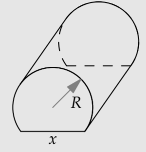
Exercise \(\PageIndex{13}\): Cylinder resting on the ground
For a solid cylinder of radius R resting on the ground (for example, a train wheel), the contact area is a rectangle. Find the scaling exponent \(\beta\) in
\[\frac{x}{R} = (\frac{\rho g R}{Y})^{\beta},\]
where x is the width of the contact strip. Then find the scaling exponent \(\gamma\) in \(F \propto \delta \gamma\), where F is the contact force and \(\delta\) is the tip compression. (In Problem 9.16, you computed the analogous scaling exponent for a sphere.)