
3.10: Valves - Modeling Dynamics
- Page ID
- 22381

\( \newcommand{\vecs}[1]{\overset { \scriptstyle \rightharpoonup} {\mathbf{#1}} } \)
\( \newcommand{\vecd}[1]{\overset{-\!-\!\rightharpoonup}{\vphantom{a}\smash {#1}}} \)
\( \newcommand{\id}{\mathrm{id}}\) \( \newcommand{\Span}{\mathrm{span}}\)
( \newcommand{\kernel}{\mathrm{null}\,}\) \( \newcommand{\range}{\mathrm{range}\,}\)
\( \newcommand{\RealPart}{\mathrm{Re}}\) \( \newcommand{\ImaginaryPart}{\mathrm{Im}}\)
\( \newcommand{\Argument}{\mathrm{Arg}}\) \( \newcommand{\norm}[1]{\| #1 \|}\)
\( \newcommand{\inner}[2]{\langle #1, #2 \rangle}\)
\( \newcommand{\Span}{\mathrm{span}}\)
\( \newcommand{\id}{\mathrm{id}}\)
\( \newcommand{\Span}{\mathrm{span}}\)
\( \newcommand{\kernel}{\mathrm{null}\,}\)
\( \newcommand{\range}{\mathrm{range}\,}\)
\( \newcommand{\RealPart}{\mathrm{Re}}\)
\( \newcommand{\ImaginaryPart}{\mathrm{Im}}\)
\( \newcommand{\Argument}{\mathrm{Arg}}\)
\( \newcommand{\norm}[1]{\| #1 \|}\)
\( \newcommand{\inner}[2]{\langle #1, #2 \rangle}\)
\( \newcommand{\Span}{\mathrm{span}}\) \( \newcommand{\AA}{\unicode[.8,0]{x212B}}\)
\( \newcommand{\vectorA}[1]{\vec{#1}} % arrow\)
\( \newcommand{\vectorAt}[1]{\vec{\text{#1}}} % arrow\)
\( \newcommand{\vectorB}[1]{\overset { \scriptstyle \rightharpoonup} {\mathbf{#1}} } \)
\( \newcommand{\vectorC}[1]{\textbf{#1}} \)
\( \newcommand{\vectorD}[1]{\overrightarrow{#1}} \)
\( \newcommand{\vectorDt}[1]{\overrightarrow{\text{#1}}} \)
\( \newcommand{\vectE}[1]{\overset{-\!-\!\rightharpoonup}{\vphantom{a}\smash{\mathbf {#1}}}} \)
\( \newcommand{\vecs}[1]{\overset { \scriptstyle \rightharpoonup} {\mathbf{#1}} } \)
\( \newcommand{\vecd}[1]{\overset{-\!-\!\rightharpoonup}{\vphantom{a}\smash {#1}}} \)
\(\newcommand{\avec}{\mathbf a}\) \(\newcommand{\bvec}{\mathbf b}\) \(\newcommand{\cvec}{\mathbf c}\) \(\newcommand{\dvec}{\mathbf d}\) \(\newcommand{\dtil}{\widetilde{\mathbf d}}\) \(\newcommand{\evec}{\mathbf e}\) \(\newcommand{\fvec}{\mathbf f}\) \(\newcommand{\nvec}{\mathbf n}\) \(\newcommand{\pvec}{\mathbf p}\) \(\newcommand{\qvec}{\mathbf q}\) \(\newcommand{\svec}{\mathbf s}\) \(\newcommand{\tvec}{\mathbf t}\) \(\newcommand{\uvec}{\mathbf u}\) \(\newcommand{\vvec}{\mathbf v}\) \(\newcommand{\wvec}{\mathbf w}\) \(\newcommand{\xvec}{\mathbf x}\) \(\newcommand{\yvec}{\mathbf y}\) \(\newcommand{\zvec}{\mathbf z}\) \(\newcommand{\rvec}{\mathbf r}\) \(\newcommand{\mvec}{\mathbf m}\) \(\newcommand{\zerovec}{\mathbf 0}\) \(\newcommand{\onevec}{\mathbf 1}\) \(\newcommand{\real}{\mathbb R}\) \(\newcommand{\twovec}[2]{\left[\begin{array}{r}#1 \\ #2 \end{array}\right]}\) \(\newcommand{\ctwovec}[2]{\left[\begin{array}{c}#1 \\ #2 \end{array}\right]}\) \(\newcommand{\threevec}[3]{\left[\begin{array}{r}#1 \\ #2 \\ #3 \end{array}\right]}\) \(\newcommand{\cthreevec}[3]{\left[\begin{array}{c}#1 \\ #2 \\ #3 \end{array}\right]}\) \(\newcommand{\fourvec}[4]{\left[\begin{array}{r}#1 \\ #2 \\ #3 \\ #4 \end{array}\right]}\) \(\newcommand{\cfourvec}[4]{\left[\begin{array}{c}#1 \\ #2 \\ #3 \\ #4 \end{array}\right]}\) \(\newcommand{\fivevec}[5]{\left[\begin{array}{r}#1 \\ #2 \\ #3 \\ #4 \\ #5 \\ \end{array}\right]}\) \(\newcommand{\cfivevec}[5]{\left[\begin{array}{c}#1 \\ #2 \\ #3 \\ #4 \\ #5 \\ \end{array}\right]}\) \(\newcommand{\mattwo}[4]{\left[\begin{array}{rr}#1 \amp #2 \\ #3 \amp #4 \\ \end{array}\right]}\) \(\newcommand{\laspan}[1]{\text{Span}\{#1\}}\) \(\newcommand{\bcal}{\cal B}\) \(\newcommand{\ccal}{\cal C}\) \(\newcommand{\scal}{\cal S}\) \(\newcommand{\wcal}{\cal W}\) \(\newcommand{\ecal}{\cal E}\) \(\newcommand{\coords}[2]{\left\{#1\right\}_{#2}}\) \(\newcommand{\gray}[1]{\color{gray}{#1}}\) \(\newcommand{\lgray}[1]{\color{lightgray}{#1}}\) \(\newcommand{\rank}{\operatorname{rank}}\) \(\newcommand{\row}{\text{Row}}\) \(\newcommand{\col}{\text{Col}}\) \(\renewcommand{\row}{\text{Row}}\) \(\newcommand{\nul}{\text{Nul}}\) \(\newcommand{\var}{\text{Var}}\) \(\newcommand{\corr}{\text{corr}}\) \(\newcommand{\len}[1]{\left|#1\right|}\) \(\newcommand{\bbar}{\overline{\bvec}}\) \(\newcommand{\bhat}{\widehat{\bvec}}\) \(\newcommand{\bperp}{\bvec^\perp}\) \(\newcommand{\xhat}{\widehat{\xvec}}\) \(\newcommand{\vhat}{\widehat{\vvec}}\) \(\newcommand{\uhat}{\widehat{\uvec}}\) \(\newcommand{\what}{\widehat{\wvec}}\) \(\newcommand{\Sighat}{\widehat{\Sigma}}\) \(\newcommand{\lt}{<}\) \(\newcommand{\gt}{>}\) \(\newcommand{\amp}{&}\) \(\definecolor{fillinmathshade}{gray}{0.9}\)Authors: Erin Knight, Matthew Russell, Dipti Sawalka, Spencer Yendell
Introduction
A valve acts as a control device in a larger system; it can be modeled to regulate the flow of material and energy within a process. There are several different kinds of valves (butterfly, ball, globe etc.), selection of which depends on the application and chemical process in consideration. The sizing of valves depends on the fluids processing unit (heat exchanger, pump etc.) which is in series with the valve. Sizing and selection of valves is discussed in the other wiki article on Valve Selection. Valves need to be modeled to perform effectively with respect to the process requirements. Important components for the modeling of control valves are:
- Flow
- Inherent Flow Characteristics
- Valve Coefficient, Cv
- Pressure Drop
- Control Valve Gain
- Rangeability
- Installed Characteristics
Efficient modeling of the valves can optimize the performance and stability of a process as well as reduce development time and cost for valve manufacturers.
In the following sections we briefly define the various variables and equations involved in modeling valves. The purpose of the following sections is to give you an overview of the equations required to model the valves for a particular system. Example problems at the end of the article have been provided to aid in the qualitative and quantitative understanding of how valves are modeled for chemical engineering processes.
Flow through a Valve
The following equation is a general equation used to describe flow through a valve. This is the equation to start with when you want to model a valve and it can be modified for different situations. The unfamiliar components such as valve coefficient and flow characteristics will be explained further.
\[F=C_{v} f(x) \sqrt{\frac{\Delta P_{v}}{s g}} \nonumber \]
with
- \(F\) is the volumetric flow rate
- \(C_v\) is the valve coefficient, the flow in gpm (gallons per minute) that flows through a valve that has a pressure drop of 1psi across the valve.
- \(ΔP_v\) is the pressure drop across the valve
- \(sg\) is the specific gravity of fluid
- \(x\) is the fraction of valve opening or valve "lift" (x=1 for max flow)
- \(f(x)\) is the flow characteristic
Flow Characteristics
The inherent flow characteristic, f(x), is key to modeling the flow through a valve, and depends on the kind of valve you are using. A flow characteristic is defined as the relationship between valve capacity and fluid travel through the valve.
There are three flow characteristics to choose from:
- \(f(x) = x\) for linear valve control
- \(f(x) = \sqrt{x}\) for quick opening valve control
- \(f(x) = R^{x − 1}\) for equal percentage valve control
- R= valve design parameter (between 20 and 50)
- note these are for a fixed pressure drop across the valve
Whereas a valve TYPE (gate, globe or ball) describes the geometry and mechanical characteristics of the valve, the valve CONTROL refers to how the flow relates to the "openness" of the valve or "x."
- Linear: flow is directly proportional to the valve lift (used in steady state systems with constant pressure drops over the valve and in liquid level or flow loops)
- Equal Percentage - equal increments of valve lift (x) produce an equal percentage in flow change (used in processes where large drops in pressure are expected and in temperature and pressure control loops)
- Quick opening: large increase in flow with a small change in valve lift (used for valves that need to be turned either on or off frequently or where instant maximum flow is required, for example, safety systems)
For the types of valves discussed in the valve selection article, the following valve characteristics are best suited:
- Gate Valves - quick opening
- Globe Valves - linear and equal percentage
- Ball Valves - quick opening and linear
- Butterfly Valves - linear and equal percentage
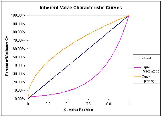
Cvmax depends on pipe characteristics and was chosen to be 110 gpm in this example. Constant pressure throughout the pipe line is assumed and the curves are accurate when the valve position is between 5% and 95% open.
Comparing the slopes of the graphs for the quick opening and equal percentage valves, we can see that a quick opening valve would experience greater change in flow with slight change in valve position in the lower flow range. The opposite is true for the higher range of flow. The equal percentage valve experiences slighter change in flow with respect to valve position in the lower range of flow.
When selecting the appropriate control valve, it is often the goal of the engineer to choose a valve that will exhibit a linear relationship between F and x over the normal operating position(s) of the valve. This linear relationship provides the most control for the operator. The flow characteristic observed through an installed valve, and all process factors considered (i.e. total pressure drop, etc.), is termed the installed flow characteristic. Therefore, it is not always the case that an inherently linear valve is desirable or even useful. An inherently linear valve is appropriate when there is a linear relationship between the valve position and the actual flow rate; however, consider the case where  and of significant value. In this case a valve with inherent equal percentage flow characteristic would be appropriate. The inherently non-linear valve would compensate for ΔPL and result in an installed linear flow characteristic.
Valve Coefficient, Cv
The valve coefficient, \(C_v\), is defined as the flow in gpm that flows through a valve with a pressure drop of 1psi across the valve (ΔPv = 1psi). Cv is an important parameter that comes up in other modeling equations. It is specific to the valve you are using.
\[C_{v}=\frac{29.9 d^{2}}{\sqrt{K}} \nonumber \]
- d = internal diameter of the pipe in inches
- K = resistance coefficient
- K is specific to the pipe shape, diameter and material. Table of typical K values
Pressure Drop
The pressure drop in the pipe line (pressure drop due to the pipe line and any other equipment in series with the valve), ΔPL, is defined as:
\[\Delta P_{L}=k_{L} \times s g \times f^{2} \nonumber \]
- f = flow through the pipe in gallons per minute [gpm]
- kL = [
 ] = constant friction coefficient for the pipe and any equipment in series with the valve
 - sg = specific gravity of the liquid
The pressure drop across the valve is defined as:
\[\Delta P_{v}=s g \frac{f^{2}}{\left(C_{v}\right)^{2}} \nonumber \]
So, the total pressure drop is described by the equation:
\[\Delta P_{o}=\Delta P_{v}+\Delta P_{L}=\left(\frac{1}{C_{v}^{2}}+k_{L}\right) s g f^{2} \nonumber \]
If the line pressure drop is negligble (constant pressure in the pipe line) then ΔPL = 0 and ΔPo = ΔPv. When ΔPL = 0 a valve with a linear flow characteristic will be desirable. When and of significant value, a valve with flow characteristics closer to an equal percentage or quick opening valve will be more desirable.
Control Valve Gain
The gain of a control valve (KL) is defined as the steady-state change in output (flow through a valve, f ) divided by the change in input (controller signal, m). The flow through a valve, f, can have units of gallons per minute (gpm), pounds per hour (lb/hr) or standard cubic feet per hour (scfh). The controller signal, m, usually has units of percent of controller output (%CO). The basic relationship for control valve gain is shown below.
\[K_{v}=\frac{d f}{d m} \nonumber \]
One objective when choosing a valve is to achieve "constant valve gain". The gain is a product of the dependence of valve position on controller output, the dependence of the flow on Cv, and the dependence of Cv on the valve position. The change in valve coefficient, Cv, with respect to valve position depends on the valve characteristics f(x).
For linear characteristics:
\[\frac{d C_{v}}{d x}=C v_{\max } \nonumber \]
For equal percentage:
\[\frac{d C_{v}}{d x}=(\ln R) C_{v} \nonumber \]
Constant Pressure Drop
The dependence of flow on the Cv depends on the pressure drop, so the equation for gain is different when there is a constant pressure drop or a variable pressure drop. If the inlet and outlet pressures do not vary with flow, the gain for either liquid or gas flow in mass units is:
- %CO = percent controller output
- W = mass flow rate
- R = valve design parameter (usually between 20 and 50)
Note: the sign is positive if the valve fails closed (air-to-open) and negative if the valve fails open (air-to-close)
Variable Pressure Drop
The valve gain for variable pressure drop is more complicated. As an example, the gain for an equal percentage is
\[K_{v}=\pm \frac{\ln \alpha}{100} \frac{f l o w}{\left(1+k_{L} C_{v}^{2}\right)} \frac{g p m}{\% C O} \nonumber \]
kL = constant friction coefficient for line, fittings, equipment, etc.
The flow term cancels some of the effect of the Cv term until the valve is fully opened, so this gain is less variable with valve opening. Therefore the installed characteristics are much more linear when compared to the inherent characteristics of an equal percentage valve.
Rangeability
Valve rangeability is defined as the ratio of the maximum to minimum controlable flow through the valve. Mathematically the maximum and minimum flows are taken to be the values when 95% (max) and 5% (min) of the valve is open.
Flow at 95% valve position Rangeability = -------------------------- Flow at 5% valve position
A smaller rangeablilty correlates to a valve that has a small range of controllable flowrates. Valves that exhibit quick opening characteristics have low rangeablilty values. Larger rangeability values correlate to valves that have a wider range of controllable flows. Linear and equal percentage valves fall into this category.
Another case to consider is when the pressure drop across the valve is independent of the flow through the valve. If this is true then the flow is proportional to CV and the rangeability can be calculated from the valve's flow characteristics equation.
Modeling Installed Valve Characteristics
When a valve is installed in series with other pieces of equipment that produce a large pressure drop in the line compared to the pressure drop across the valve, the actual valve characteristics deviate from the inherent characteristics. At large in-line pressure drops the pressure drop, and consequently the valve coefficient, varies with flow through the valve. These changes can cause changes in the rangeabilty and distorts inherent valve characteristics.
In the following Microsoft® Excel model, the variation from inherent valve characteristics is illustrated. A number of parameters can be changed to match the flow conditions through a valve. This model simulates both linear and equal percentage valve characteristics. To more clearly demonstrate the deviation from inherent characteristics; simply change the CVmax value of the valve. Notice how the installed valve characteristics and valve rangeability change drastically.
Installed Valve Characteristcs Model
Special Considerations for the Equation describing Flow Through a Valve
Compressible Fluids
- Manufacturers such as Honeywell, DeZurik, Masoneilan and Fischer Controls have modified the flow equation to model compressible flows. The equations are derived from the equation for flow through a valve but include unit conversion factors and corrections for temperature and pressure, which affect the density of the gas. It is important to remember to account for these factors if you are working with a compressible fluid such as steam.
Accuracy
- This equation, and its modified forms, is most accurate for water, air or steam using conventional valves installed in straight pipes. If you are dealing with non-Newtonian, viscous or two phase systems the calculations will be less accurate.
Example 1: Verbal Model of a Control Valve
Problem Statement:
Verbally model a fail open control valve positioned as a safety measure on a reactor processing an exothermic reaction.
Solution
- Describe the Process: In the fail-open control valve a quick opening valve opens with a failure signal. Open is its default position once the signal goes off.
- Identify Process Objectives and Constraints: A fail-open control valve is a safety measure. For example, if your cooling heat exchanger fails and the reactor starts to heat up and produce excess gases, the fail-open control valve would release excess gasses before pressure builds up to produce an explosion. The size of the valve is a constraint because it limits how much fluid can escape. The valve size determines the maximum flow rate. The shape and angles of the valve are modeling constraints. Sudden and gradual contraction or enlargement of the pipe diameter inside the valve and the connecting piping, will change the resistance coefficient and therefore the maximum velocity.
- Identify Significant Disturbances: Significant internal disturbances include the escalating pressure and temperature as the exothermic reaction gets out of control.
- Determine the Type and Location of Sensors: A pressure sensor would be located in the tank with the control valve that would provide the signal to the fail-open control valve. To achieve redundancy, a temperature sensor would be located on the heat exchanger to signal failure of the cooling apparatus.
- Determine the Location of Control Valves: A fail-open control valve (or multiple valves) would be placed on the top of the tank to allow exit of the gasses in the processing unit.
- Apply a Degree-of-Freedom Analysis: The only manipulated variable is the valve coefficient. This depends on the valve’s diameter and resistance coefficient K. The control objective is the maximum flow rate. The pressure drop will vary according to the failure. Therefore there is one degree of freedom.
- Implement Energy Management: This doesn’t apply to our confined example, but in a larger system we could install a backup cooler if this reaction were truly dangerous.
- Control Process Production Rate and Other Operating Parameters: The exit flow rate can not exceed the maximum flow rate through the control valve.
- Handle Disturbances and Process Constraints: If our first control valve fails to sufficiently lower the tank pressure, a signal would be sent to a second valve and depending on the reaction, a backup cooling system. A secondary cooling system would be too expensive for many cases, but if you were dealing with a nuclear reactor or something highly explosive it may be worth the investment.
- Check Component Balances: Does not apply. Preventing accumulation is the point of this control valve.
- Apply Process Optimization: Our manipulatable variable is choosing a valve with a specific Cv. The valve should be able to withstand extreme temperatures and high pressures. It would be a gate valve, which opens completely upon failure. For other sizing concerns refer to “Valve Sizing.”
A new valve is being installed downstream from a water pump. The friction coefficient of the pump and associated piping that will be in series with the new valve is
\[k_{L}=1.4 \times 10^{-4}\left(\frac{p s i}{g p m^{2}}\right). \nonumber \]
The flow through the line from the pump is 300 gpm. The desired pressure drop across the valve is 4 psi. A high level of control is desired for the flow through the new valve. Two valves are being considered, one has an inherent linear characteristic, the other is equal percentage (α=50). From the manufacturer’s literature, both have a CVmax value of 200. Use the Installed Valve Characteristics Model to determine which valve has a higher range of controllable flows values.
Solution
Note that the pressure drop across the pipe is 13.5psi, which is significantly larger than the pressure drop across the valve (4 psi). These conditions indicate that the characteristic flow through the valves may not match the inherent characteristics. This is verified by the plots and also by the calculated rangeability values shown in the valve model spreadsheet. The equal percentage valve has a higher rangeabilty value, corresponding to a higher range of controllable flows.
References
- Bequette, B. Wayne. Process Control Modeling, Design, and Simulation, Upper Saddle River, New Jersey: Prentice Hall.
- Crane Co. Flow of Fluids Through Valves, Fittings, and Pipe, Joliet, IL: CRANE.
- "Friction Losses in Pipe Fittings"(PDF), Western Dynamics, LLC., retrieved September 11, 2006.
- Perry, R. H., and D. Green (ed). Perry's Chemical Engineering Handbook, 7th ed. New York: McGraw-Hill.
- Seborg, Dale E., Thomas F. Edgar, Duncan A Mellichamp. Process Dynamics and Control, New York: John Wiley & Sons.
- Smith, Carlos A., Armando B. Corripio. Principles and Practice of Automatic Process Control, 3rd ed. New York: John Wiley & Sons.
- "Valve Sizing and Selection." The Chemical Engineers' Resource Page. 1442 Goswick Ridge Road, Midlothian, VA 23114. retrieved Sept 24, 2006.