
7.2: First-order Differential Equations
- Page ID
- 22404

\( \newcommand{\vecs}[1]{\overset { \scriptstyle \rightharpoonup} {\mathbf{#1}} } \)
\( \newcommand{\vecd}[1]{\overset{-\!-\!\rightharpoonup}{\vphantom{a}\smash {#1}}} \)
\( \newcommand{\dsum}{\displaystyle\sum\limits} \)
\( \newcommand{\dint}{\displaystyle\int\limits} \)
\( \newcommand{\dlim}{\displaystyle\lim\limits} \)
\( \newcommand{\id}{\mathrm{id}}\) \( \newcommand{\Span}{\mathrm{span}}\)
( \newcommand{\kernel}{\mathrm{null}\,}\) \( \newcommand{\range}{\mathrm{range}\,}\)
\( \newcommand{\RealPart}{\mathrm{Re}}\) \( \newcommand{\ImaginaryPart}{\mathrm{Im}}\)
\( \newcommand{\Argument}{\mathrm{Arg}}\) \( \newcommand{\norm}[1]{\| #1 \|}\)
\( \newcommand{\inner}[2]{\langle #1, #2 \rangle}\)
\( \newcommand{\Span}{\mathrm{span}}\)
\( \newcommand{\id}{\mathrm{id}}\)
\( \newcommand{\Span}{\mathrm{span}}\)
\( \newcommand{\kernel}{\mathrm{null}\,}\)
\( \newcommand{\range}{\mathrm{range}\,}\)
\( \newcommand{\RealPart}{\mathrm{Re}}\)
\( \newcommand{\ImaginaryPart}{\mathrm{Im}}\)
\( \newcommand{\Argument}{\mathrm{Arg}}\)
\( \newcommand{\norm}[1]{\| #1 \|}\)
\( \newcommand{\inner}[2]{\langle #1, #2 \rangle}\)
\( \newcommand{\Span}{\mathrm{span}}\) \( \newcommand{\AA}{\unicode[.8,0]{x212B}}\)
\( \newcommand{\vectorA}[1]{\vec{#1}} % arrow\)
\( \newcommand{\vectorAt}[1]{\vec{\text{#1}}} % arrow\)
\( \newcommand{\vectorB}[1]{\overset { \scriptstyle \rightharpoonup} {\mathbf{#1}} } \)
\( \newcommand{\vectorC}[1]{\textbf{#1}} \)
\( \newcommand{\vectorD}[1]{\overrightarrow{#1}} \)
\( \newcommand{\vectorDt}[1]{\overrightarrow{\text{#1}}} \)
\( \newcommand{\vectE}[1]{\overset{-\!-\!\rightharpoonup}{\vphantom{a}\smash{\mathbf {#1}}}} \)
\( \newcommand{\vecs}[1]{\overset { \scriptstyle \rightharpoonup} {\mathbf{#1}} } \)
\(\newcommand{\longvect}{\overrightarrow}\)
\( \newcommand{\vecd}[1]{\overset{-\!-\!\rightharpoonup}{\vphantom{a}\smash {#1}}} \)
\(\newcommand{\avec}{\mathbf a}\) \(\newcommand{\bvec}{\mathbf b}\) \(\newcommand{\cvec}{\mathbf c}\) \(\newcommand{\dvec}{\mathbf d}\) \(\newcommand{\dtil}{\widetilde{\mathbf d}}\) \(\newcommand{\evec}{\mathbf e}\) \(\newcommand{\fvec}{\mathbf f}\) \(\newcommand{\nvec}{\mathbf n}\) \(\newcommand{\pvec}{\mathbf p}\) \(\newcommand{\qvec}{\mathbf q}\) \(\newcommand{\svec}{\mathbf s}\) \(\newcommand{\tvec}{\mathbf t}\) \(\newcommand{\uvec}{\mathbf u}\) \(\newcommand{\vvec}{\mathbf v}\) \(\newcommand{\wvec}{\mathbf w}\) \(\newcommand{\xvec}{\mathbf x}\) \(\newcommand{\yvec}{\mathbf y}\) \(\newcommand{\zvec}{\mathbf z}\) \(\newcommand{\rvec}{\mathbf r}\) \(\newcommand{\mvec}{\mathbf m}\) \(\newcommand{\zerovec}{\mathbf 0}\) \(\newcommand{\onevec}{\mathbf 1}\) \(\newcommand{\real}{\mathbb R}\) \(\newcommand{\twovec}[2]{\left[\begin{array}{r}#1 \\ #2 \end{array}\right]}\) \(\newcommand{\ctwovec}[2]{\left[\begin{array}{c}#1 \\ #2 \end{array}\right]}\) \(\newcommand{\threevec}[3]{\left[\begin{array}{r}#1 \\ #2 \\ #3 \end{array}\right]}\) \(\newcommand{\cthreevec}[3]{\left[\begin{array}{c}#1 \\ #2 \\ #3 \end{array}\right]}\) \(\newcommand{\fourvec}[4]{\left[\begin{array}{r}#1 \\ #2 \\ #3 \\ #4 \end{array}\right]}\) \(\newcommand{\cfourvec}[4]{\left[\begin{array}{c}#1 \\ #2 \\ #3 \\ #4 \end{array}\right]}\) \(\newcommand{\fivevec}[5]{\left[\begin{array}{r}#1 \\ #2 \\ #3 \\ #4 \\ #5 \\ \end{array}\right]}\) \(\newcommand{\cfivevec}[5]{\left[\begin{array}{c}#1 \\ #2 \\ #3 \\ #4 \\ #5 \\ \end{array}\right]}\) \(\newcommand{\mattwo}[4]{\left[\begin{array}{rr}#1 \amp #2 \\ #3 \amp #4 \\ \end{array}\right]}\) \(\newcommand{\laspan}[1]{\text{Span}\{#1\}}\) \(\newcommand{\bcal}{\cal B}\) \(\newcommand{\ccal}{\cal C}\) \(\newcommand{\scal}{\cal S}\) \(\newcommand{\wcal}{\cal W}\) \(\newcommand{\ecal}{\cal E}\) \(\newcommand{\coords}[2]{\left\{#1\right\}_{#2}}\) \(\newcommand{\gray}[1]{\color{gray}{#1}}\) \(\newcommand{\lgray}[1]{\color{lightgray}{#1}}\) \(\newcommand{\rank}{\operatorname{rank}}\) \(\newcommand{\row}{\text{Row}}\) \(\newcommand{\col}{\text{Col}}\) \(\renewcommand{\row}{\text{Row}}\) \(\newcommand{\nul}{\text{Nul}}\) \(\newcommand{\var}{\text{Var}}\) \(\newcommand{\corr}{\text{corr}}\) \(\newcommand{\len}[1]{\left|#1\right|}\) \(\newcommand{\bbar}{\overline{\bvec}}\) \(\newcommand{\bhat}{\widehat{\bvec}}\) \(\newcommand{\bperp}{\bvec^\perp}\) \(\newcommand{\xhat}{\widehat{\xvec}}\) \(\newcommand{\vhat}{\widehat{\vvec}}\) \(\newcommand{\uhat}{\widehat{\uvec}}\) \(\newcommand{\what}{\widehat{\wvec}}\) \(\newcommand{\Sighat}{\widehat{\Sigma}}\) \(\newcommand{\lt}{<}\) \(\newcommand{\gt}{>}\) \(\newcommand{\amp}{&}\) \(\definecolor{fillinmathshade}{gray}{0.9}\)Introduction
We consider the general first-order differential equation:
\[\tau \dfrac{d y(t)}{d t}+y(t)=x(t) \nonumber \]
The general solution is given by:
\[y(t)=y_{0} e^{-\left(t-t_{0}\right) / \tau}+\dfrac{e^{-\left(t-t_{0}\right) / \tau}}{\tau} \int_{t_{0}}^{t} x\left(t^{\prime}\right) e^{\left(t^{\prime}-t_{0}\right) / \tau} d t^{\prime} \nonumber \]
where \(y_{0}=y \left(t-t_{0}\right)\). Note that \(t^{\prime}\) is used to be distinguished from the upper limit \(t\) of the integral.
To obtain the general solution, begin with the first order differential equation:
\[\tau \dfrac{d y(t)}{d t}+y(t)=x(t) \nonumber \]
Divide both sides by \(\tau\):
\[\dfrac{d y(t)}{d t}+\dfrac{1}{\tau} y(t)=\dfrac{1}{\tau} x(t) \nonumber \]
Rewrite the LHS in condensed form using the integrating factor \(e^{ − t / τ}\):
\[e^{-t / \tau} \dfrac{d}{d t}\left[e^{t / \tau} y(t)\right]=\dfrac{1}{\tau} x(t) \nonumber \]
Notice how a chain differentiation will return the LHS to the previous form
Simplify:
\[\dfrac{d}{d t}\left[e^{t / \tau} y(t)\right]=\dfrac{1}{\tau} x(t) e^{t / \tau} \nonumber \]
Integrate both sides:
\[e^{t / \tau} y(t)-e^{t_{0} / \tau} y\left(t_{0}\right)=\dfrac{1}{\tau} \int_{t_{0}}^{t} x\left(t^{\prime}\right) e^{t^{\prime} / \tau} d t^{\prime} \nonumber \]
Solve for \(y(t)\):
\[y(t)=y_{0} e^{-\left(t-t_{0}\right) / \tau}+\dfrac{e^{-t / \tau}}{\tau} \int_{t_{0}}^{t} x\left(t^{\prime}\right) e^{t^{\prime} / \tau} d t^{\prime} \nonumber \]
Consider:
\[\dfrac{d y(t)}{d t}=x(t) \nonumber \]
Multiplying both sides by \(dt\) gives:
\[\int_{t_{0}}^{t} \dfrac{d y d t}{d t}=\int_{t_{0}}^{t} x\left(t^{\prime}\right) d t^{\prime} \nonumber \]
The general solution is given as:
\[y(t)=y_{0}+\int_{t_{0}}^{t} x\left(t^{\prime}\right) d t^{\prime} \nonumber \]
Now Consider:
\[\dfrac{d y(t)}{d t}=-a y(t) \nonumber \]
Dividing both sides by \(y(t)\) gives:
\[\dfrac{1}{y(t)} \dfrac{d y(t)}{d t}=-a \nonumber \]
which can be rewritten as:
\[\dfrac{d}{d t}[\ln (y(t))]=-a \nonumber \]
Multiplying both sides by \(dt\), integrating, and setting both sides of the equation as exponents to the exponential function gives the general solution:
\[y(t)=y_{0} e^{-a\left(t-t_{0}\right)} \nonumber \]
Now Consider:
\[\dfrac{d y(t)}{d t}=-a y(t)+x(t) \nonumber \]
The detailed solution steps are as follows:
1. Separate \(y(t)\) and \(x(t)\) terms
\[\dfrac{d y(t)}{d t}+a y(t)=x(t) \nonumber \]
2. Rewrite the LHS in condensed form using the "integrating factor" \(e^{ − at}\)
\[e^{-a t} \dfrac{d\left(e^{a t} y(t)\right)}{d t}=x(t) \nonumber \]
Notice how a chain differentiation will return the LHS to the form written in step 1
3. Divide both sides by \(e^{− at}\)
\[\dfrac{d\left(e^{a t} y(t)\right)}{d t}=e^{a t} x(t) \nonumber \]
4. Multiply both sides by \(dt\) and integrate
\[e^{a t} y(t)-e^{a t_{0}} y_{0}=\int_{t_{0}}^{t} x\left(t^{\prime}\right) e^{a t^{\prime}} d t^{\prime} \nonumber \]
The general solution is given as:
\[y(t)=y_{0} e^{-a\left(t-t_{0}\right)}+e^{-a t} \int_{t_{0}}^{t} x\left(t^{\prime}\right) e^{a\left(t^{\prime}-t_{0}\right)} d t^{\prime} \nonumber \]
Step Function Simplification
\[\tau \dfrac{d y(t)}{d t}+y(t)=x(t) \nonumber \]
For \(x(t)=\Theta\left(t-t_{0}\right)\), which is the step function and \(y_{0}=0\)
That is, \(x(t)=1\) for \( t_0 > t_o\) and \(x(t)=0\) otherwise:
The previously derived general solution:
\[y(t)=y_{0} e^{-\left(t-t_{0}\right) / \tau}+\dfrac{e^{-\left(t-t_{0}\right) / \tau}}{\tau} \int_{t_{0}}^{t} x\left(t^{\prime}\right) e^{\left(t^{\prime}-t_{0}\right) / \tau} d t^{\prime} \nonumber \]
reduces to:
\[y(t)=e^{-\left(t-t_{0}\right) / \tau} \nonumber \]
since the integral equals 1.
The quantity \(\tau\) can be seen to be the time constant whereby \(y(t)\) drops to \(1/e\) of its original value
Consider the differential equation
\[\dfrac{d y(t)}{d t}=-0.5 y(t)+x(t) \nonumber \]
where \(x(t)=2+0.01 t\)
Assuming \(y_o =0\), what is the behavior of \(y(t)\)?
Solution
General solution was derived previously as:
\[y(t)=y_{0} e^{-a\left(t-t_{0}\right)}+e^{-a t} \int_{t_{0}}^{t} x\left(t^{\prime}\right) e^{a\left(t^{\prime}-t_{0}\right)} d t^{\prime} \nonumber \]
For \(a=0.5\) and \(y_o = 0\), while setting \(t_o=0\), the solution reduces to:
\[y(t)=e^{-0.5 t} \int_{0}^{t}\left(2+0.01 t^{\prime}\right) e^{0.5\left(t^{\prime}\right)} d t^{\prime} \nonumber \]
The following link may be referred to for integral tables: S.O.S. Math
Simplifying the solution gives the following:
\[y(t)=\dfrac{\left.\left(e^{-0.5 t}\right)\left((x+198)\left(e^{0.5 t}\right)-198\right)\right)}{50} \nonumber \]
Plotting this function displays the following behavior:
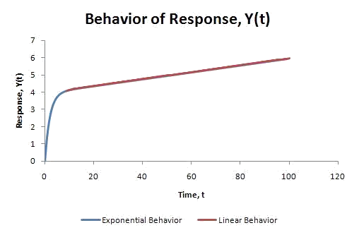
As can be seen clearly from the graph, initially the systemic response shows more exponential characteristics. However, as time progresses, linear behavior dominates.