12.5: Understanding MIMO Control Through Two Tanks Interaction

We have been familiar with the models of single surge tank manipulated by first order process and two tanks in series manipulated by second order process, both of which are typical examples of Single Input Single Output (SISO) control. However, in the real chemical processes, there are always interations between the reactors. The following page will discuss the two tanks model by taking into consideration the interaction between the two tanks. To manipulate this model, we need to use Multiple Input Multiple Output (MIMO) control, which will add more complexity in understanding the overall process.

Two Tanks Interaction Model

The following figure, Figure 1, demonstrates how two tanks model works to interact each other. From Figure 1, we can see that the input of Tank1, x1, not only affects the level in Tank1, but also affects that in Tank2. The same goes for the input of Tank2, x2. We use the resistance, R3, to account for the interaction between the two tanks.

Figure 1: Two tanks interaction model

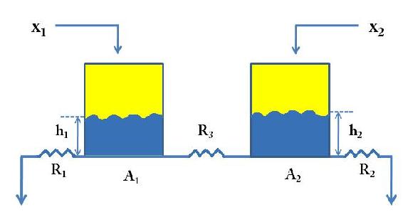
In the above figure,

• \(x_1\) = Input of Tank1
• \(x_2\) = Input of Tank2
• \(A_1\) = Cross section area of Tank1
• \(A_2\) = Cross section area of Tank2
• \(h_1\) = Level of Tank1
• \(h_2\) = Level of Tank2
• \(R_1\) = Resistance of Tank1
• \(R_2\) = Resistance of Tank2
• \(R_3\) = Interaction Resistance

Mathematical Equations for the Process

Now, we will derive the mathematical equations to describe the process, now we assume the direction of the flow goes from Tank1 to Tank2:

To begin with, we write down the governing equation for each of the tanks, taking into consideration the interaction term:

\[A_{1} \dfrac{d h_{1}}{d t}=x_{1}-\dfrac{h_{1}}{R_{1}} d t-\dfrac{\left(h_{1}-h_{2}\right)}{R_{3}}=x_{1}+h_{1}\left(-\dfrac{1}{R_{1}}-\dfrac{1}{R_{3}}\right)+h_{2}\left(\dfrac{1}{R_{3}}\right) \nonumber \]

\[A_{2} \dfrac{d h_{2}}{d t}=x_{2}-\dfrac{h_{2}}{R_{2}} d t+\dfrac{\left(h_{1}-h_{2}\right)}{R_{3}}=x_{2}+h_{2}\left(-\dfrac{1}{R_{2}}-\dfrac{1}{R_{3}}\right)+h_{1}\left(\dfrac{1}{R_{3}}\right) \nonumber \]

Under steady state, the time derivatives, i.e. the left hand side of the above equations, go to zero:

\[0=x_{1}(0)+h_{1}(0)\left(-\dfrac{1}{R_{1}}-\dfrac{1}{R_{3}}\right)+h_{2}(0)\left(\dfrac{1}{R_{3}}\right) \nonumber \]

\[0=x_{2}(0)+h_{1}(0)\left(\dfrac{1}{R_{3}}-\dfrac{1}{R_{3}}\right)+h_{2}(0)\left(-\dfrac{1}{R_{2}}-\dfrac{1}{R_{3}}\right) \nonumber \]

Now, we define the deviation variables as follows:

• \(X_1 = x_1 − x_1(0)\)
• \(Y_1 = h_1 − h_1(0)\)
• \(X_2 = x_2 − x_2(0)\)
• \(Y_2 = h_2 − h_2(0)\)

Set \(y_1=h_1\) and \(y_2=h_2\), we can obtain the following equations:

\[A_{1} \dfrac{d y_{1}}{d t}=\dfrac{x_{1}}{A_{1}}+y_{1}\left(-\dfrac{1}{A_{1} R_{1}}-\dfrac{1}{A_{1} R_{3}}\right)+y_{2}\left(\dfrac{1}{A_{1} R_{3}}\right) \nonumber \]

\[A_{2} \dfrac{d y_{2}}{d t}=\dfrac{x_{2}}{A_{1}}+y_{1}\left(\dfrac{1}{A_{2} R_{3}}\right)+y_{2}\left(-\dfrac{1}{A_{2} R_{2}}-\dfrac{1}{A_{2} R_{3}}\right) \nonumber \]

It will be more general if we write down the above equations into a form of Matrix:

\[\left[\begin{array}{c}
\dot{y}_{1} \\
\dot{y}_{2}
\end{array}\right]=\left[\begin{array}{cc}
\dfrac{1}{A_{1}} & 0 \\
0 & \dfrac{1}{A_{2}}
\end{array}\right]\left[\begin{array}{c}
x_{1} \\
x_{2}
\end{array}\right]+\left[\begin{array}{cc}
-\dfrac{1}{A_{1} R_{1}}-\dfrac{1}{A_{1} R_{2}} & \dfrac{1}{A_{1} R_{3}} \\
\dfrac{1}{A_{2} R_{3}} & -\dfrac{1}{A_{2} R_{2}}-\dfrac{1}{A_{2} R_{3}}
\end{array}\right]\left[\begin{array}{c}
y_{1} \\
y_{2}
\end{array}\right] \nonumber \]

We can represent the above equation using the following equation:

\[\begin{array}{c}
\vec{y}=\overrightarrow{\vec{B}} \vec{x}+\overrightarrow{\vec{A}} \vec{y} \\
\vec{y}-\vec{A} \vec{y}=\overrightarrow{\vec{B}} \vec{x} \\
\vec{x}=\left(\vec{B}^{-1}\right)\left(\dfrac{\partial}{\partial t}-\overrightarrow{\vec{A}}\right) \vec{y}=\overrightarrow{\vec{G}_{p}}^{-1} \vec{y}
\end{array} \nonumber \]

Invert the above equation:

Now, set

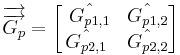
We get the following equation:

\[\left[\begin{array}{c}
y_{1} \\
y_{2}
\end{array}\right]=\left[\begin{array}{cc}
\hat{G}_{p 1,1} & \hat{G}_{p 1,2} \\
\hat{G}_{p 2,1} & \hat{G}_{p 2,2}
\end{array}\right]\left[\begin{array}{c}
x_{1} \\
x_{2}
\end{array}\right]\]

Control Diagram

Figure 2: Contol Diagram for Two tanks interaction model.

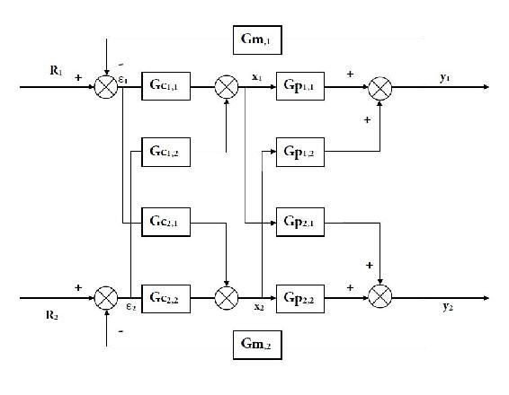
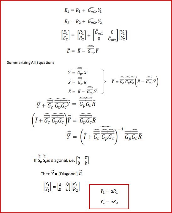
Decouple the process