5.1: Root Locus Fundamentals

 

Root Locus

The root locus (RL) constitutes a graph of the closed-loop root locations, with variation in static feedback controller gain, \(K\).

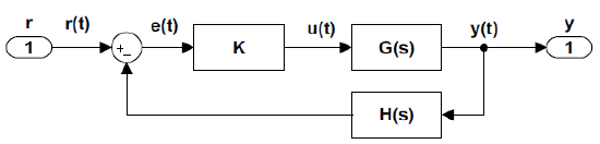
In order to develop the RL concepts, we consider a typical feedback control system (Figure 5.1), where \(K\) represents a controller, \(G(s)\) is the plant transfer function, and \(H(s)\) is the sensor transfer function. Unless noted otherwise, unity-gain feedback (\(H(s)=1\)) is assumed.

Figure \(\PageIndex{1}\): Feedback control system with plant \(G(s)\), sensor \(H(s)\), and a static gain controller represented by \(K\).

The loop gain for the feedback loop includes the controller, the plant, and the sensor transfer functions, and is given as: \[L(s)=KG(s)H(s)=KGH(s) \nonumber \]

The characteristic polynomial of the closed-loop system is defined as: \[\Delta (s,K)=1+KGH(s) \nonumber \]

The roots of \(\Delta (s,K)\) vary with the controller gain, \(K\), and are plotted for different values of \(K\). The loci of all such roots locations, as \(K\) varies from \(0\to \infty ,\) constitutes the root locus plot of the loop transfer function.

Example \(\PageIndex{1}\)

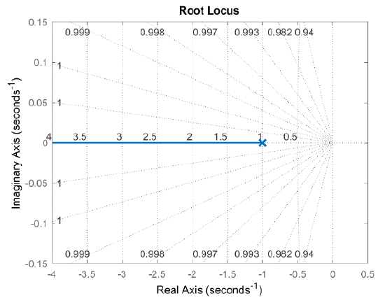
Let \(G(s)=\frac{1}{s+1} ,\; H(s)=1\); the closed-loop characteristic polynomial is given as: \(\Delta (s)=s+1+K.\) The polynomial has a single root at \(s_{1} =-1-K\).

A short table of closed-loop root for different values of \(K\) is given below:

\(K\)	\(0\)	\(1\)	\(2\)	\(5\)	\(10\)
Closed-loop root	\(-1\)	\(-2\)	\(-3\)	\(-6\)	\(-11\)

The root locus plot, as \(K\) varies from \(0\) to \(\infty\), traces a line that proceeds from \(\sigma =-1\) along the negative real-axis to infinity (Figure 5.1.2). The overlaid grid shows the damping ratio of the closed-loop root (\(\zeta=1\) in this case).

Figure \(\PageIndex{2}\): The root locus plot for \(G(s)=\frac{1}{s+1} ,\; H(s)=1\)

pkg load control
s=tf('s');
Gs=1/(s+1);
rlocus(Gs)

The MATLAB Control Systems Toolbox provides the ‘rlocus’ command to plot the root locus of the loop transfer function. The ‘rlocus’ command is invoked after defining a dynamic system object using ‘tf’ or ‘zpk’ command.

The ‘grid’ command adds constant damping ratio and constant natural frequency contours to the RL plot. These contours help design a static controller for desired values of those parameters. 

Example \(\PageIndex{2}\)

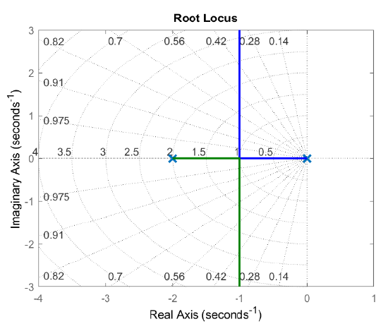
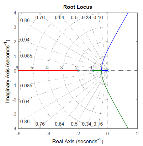
Let \(G(s)=\frac{1}{s(s+2)} ,\; \; H(s)=1\). The closed-loop characteristic polynomial is given as: \(\Delta (s,K)=s^{2} +2s+K.\)

The roots of the characteristic polynomial are given as: \(s_{1,2}=-1\pm \sqrt{1-K}\) for \(K\le 1\), and as \(s_{1,2} =-1\pm j\sqrt{K-1}\) for \(K>1\). The roots for selected values of \(K\) are tabulated below.

\(K\)	\(0\)	\(1\)	\(2\)	\(10\)
Closed-loop roots	\(-1,-2\)	\(-1,-1\)	\(-1\pm j1\)	\(-1\pm j3\)

The loci of these roots, as \(K\) varies from \(0\to \infty\), comprise two branches that commence at the open-loop (OL) poles located at \(\{ 0,\; -2\}\), proceed inward along the real-axis to meet at \(\sigma =-1\), then split and extend along the \(\sigma =-1\) line to \(s=-1\pm j\infty\) (Figure 5.2). These directions are called the RL asymptotes.

Figure \(\PageIndex{3}\): The root locus plot for \(G(s)=\frac{1}{s(s+2)} ,\; \; H(s)=1\).

pkg load control
s=tf('s');
Gs=1/s/(s+1);
rlocus(Gs)

The RL plot can be extended to negative values of \(K\), i.e., \(K\in (-\infty ,\; \infty )\), and is called generalized root locus. 

Root Locus Rules

All RL plots share a few common properties, referred as the root locus rules. The prominent rules are described below.

In the following, it is assumed that the loop transfer function, \(KGH(s)\), is proper, has \(n\) open loop (OL) poles and \(m\le n\) finite OL zeros. The remaining \(n-m\) zeros are assumed to lie at infinity.

1. The RL has \(n\) branches and \(n-m\) asymptotes (assumed RL directions for large \(K\)). The RL branches commence at the OL poles (for \(K=0\)); of these, \(m\) branches terminate at the OL zeros (as \(K\to \infty\)); the remaining \(n-m\) branches follow the RL asymptotes to infinity (as \(K\to \infty\)).
2. The real-axis locus, indicating real roots of the characteristic polynomial, lies to the left of an odd number of poles and zeros of \(KGH(s)\) for \(\left(K>0\right)\), and to the right of an odd number of poles and zeros for \(\left(K<0\right)\).
3. The real-axis locus separating a pair of OL poles contains a break-away point where the two RL branches split; the real-axis locus separating two OL zeros, contains a break-in point where the two branches meet. The break points for both \(K>0\) and \(K<0\) are found among the solutions to the equation: \(\sum \frac{1}{\sigma -p_{i} } -\sum \frac{1}{\sigma -z_{i} } =0\).
4. The RL asymptotes, assume angles: \(\phi _{a} =\frac{2k+1}{n-m} (180^{\circ } ),\; k=0,\; 1,\cdots ,n-m-1\), (for\(K>0\)), and angles: \(\phi _{a} =\frac{2k+1}{n-m} (360^{\circ })\),  \(k=0,\; 1,\cdots ,n-m-1\) (for \(K<0\)). These asymptotes intersect at a common point on the real-axis, given as: \(\sigma _a =\frac{\sum p_{i} -\sum z_{i} }{n-m}\).
5. The RL plot is symmetric with respect to the real-axis (this is a consequence of the fact that the complex roots of a real polynomial occur in conjugate pairs).

The above rules suffice to sketch the RL plot for low-order plants. Additional rules for refining the RL plot may be added.

Example \(\PageIndex{3}\)

Let \(KGH(s)=\frac{K(s+3)}{s(s+2)}\); hence, \(n=2,\ \ m=1\).The closed-loop characteristic polynomial is formed as: \(\mathit{\Delta}\left(s,K\right)=s^2+\left(K+2\right)s+3K\).

The RL plot is sketched as follows:

1. The RL has two branches that commence at the OL poles at \(0,-2\) (for \(K=0)\); one branch terminates at the finite OL zero at \(s=-3\); the other branch follows the RL asymptote as \(K\to \infty\).
2. The real-axis locus lies in the intervals: \(\sigma \in \left[-2,0\right]\cup (-\infty ,-3]\) (for \(K>0)\).
3. The real-axis break points are defined by: \(\frac{1}{\sigma } +\frac{1}{\sigma +2} =\frac{1}{\sigma +3}\), or \({\sigma }^2+6\sigma +6=0\); the solutions include: \(\sigma =-1.27\) (break-away) and \(-4.73\) (break-in).
4. The asymptote angle is given as: \(\pm 180^{\circ }\) (for \(K>0\)), with intersection at: \(\sigma _{a} =1\).

The resulting RL plot (for \(K>0\)) is shown in Figure 5.1.4.

Figure \(\PageIndex{4}\): The root locus plot for \(G(s)=\frac{(s+3)}{s(s+2)}\).

pkg load control
s=tf('s');
Gs=(s+3)/s/(s+2);
rlocus(Gs)

                                                                               
                                  Root Locus of Gs                             
                                                                               
         |-----------------------------------------------------------------|   
         |   +      +       +      +      +       ++------$$$$$$$---------+|   
     1.5 |-+&&&&&&&&&&&&&&&&&&&&&&&&&&&&&&&&&&&&&&&|###?#$$locus$$       +||   
         |   &      &       &      &      &       &|   B$$ open loop poles||   
       1 |-+&&&&&&&&&&&&&&&&&&&&&&&&&&&&&&&&&&&&&&&+---F$--zeros--$-------+|   
         |   &      &       &      &      &       &    $ &       &$$    &  |   
     0.5 |-+&&&&&&&&&&&&&&&&&&&&&&&&&&&&&&&&&&&&&&&&&&&$&&&&&&&&&&&$&&&&&+-|   
         |   &      &       &      &      &       &    $ &       & $    &  |   
       0 |**##########################################$$$$$$$F***B#$$$$$B**|   
         |   &      &       &      &      &       &   #  &       & #    &  |   
         |   &      &       &      &      &       &    # &       & #    &  |   
    -0.5 |-+&&&&&&&&&&&&&&&&&&&&&&&&&&&&&&&&&&&&&&&&&&&#&&&&&&&&&&&#&&&&&+-|   
         |   &      &       &      &      &       &    # &       &##    &  |   
      -1 |-+&&&&&&&&&&&&&&&&&&&&&&&&&&&&&&&&&&&&&&&&&&&##&&&&&&&&&#&&&&&&+-|   
         |   &      &       &      &      &       &     ##       ##     &  |   
    -1.5 |-+&&&&&&&&&&&&&&&&&&&&&&&&&&&&&&&&&&&&&&&&&&&&&##&&&&&##&&&&&&&+-|   
         |   +      +       +      +      +       +      +#######+      +  |   
         |-----------------------------------------------------------------|   
            -16    -14     -12    -10    -8      -6     -4      -2      0      
                          Real Axis     gain = [0, 17.4235]                    
                                                                               

Example \(\PageIndex{4}\)

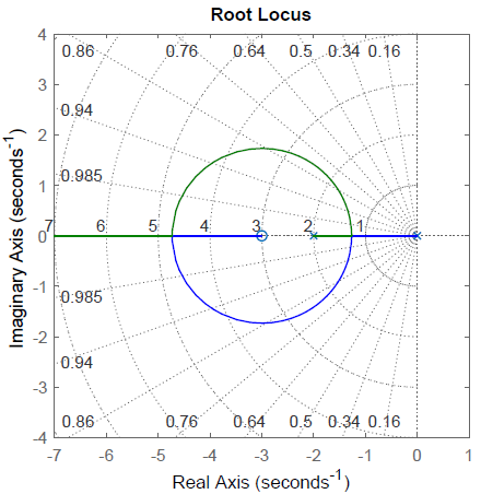
Let \(KGH(s)=\frac{K}{s(s+1)(s+2)}\); then, \(n=3,\ m=0\). The closed-loop characteristic polynomial is formed as: \(\Delta (s)=s^{3} +3s^{2} +2s+K\).

The RL plot is sketched as follows:

1. The RL has three branches that commence at the OL poles at \(s=0,-1,-2\) (for \(K=0)\); the branches follow RL asymptotes as \(K\to \infty\).
2. The real-axis locus lies along \(\sigma \in \left[-1,0\right]\) (for \(K>0)\).
3. The break points are given as the solution to: \(\frac{1}{\sigma } +\frac{1}{\sigma +1} +\frac{1}{\sigma +2} =0\), which reduces to: \(3\sigma ^{2} +6\sigma +2=0\), and has solutions at \(\sigma =-0.38,\; -2.62\). The first solution is a break-away point for \(K>0\); the second one is the break-in point for \(K<0\).
4. The asymptote angles are given as: \(\pm 60^{\circ } ,180^{\circ }\) (for \(K>0\)); their common intersection point is at: \(\sigma _a =-\frac{3}{3} =-1\).

The resulting RL plot (for \(K>0\)) is shown in Figure 5.1.5.

Figure \(\PageIndex{5}\): The root locus plot for \(G(s)=\frac{1}{s(s+1)(s+2)}\).

pkg load control
s=tf('s');
Gs=1/s/(s+1)/(s+2);
rlocus(Gs)

                                                                               
                                 Root Locus of Gs                              
                                                                               
       |-------------------------------------------------------------------|   
       |    +            +            +            +----------------**&&&-+|   
     2 |-+*****************************************|###?###asymptote&&&  +||   
       |    *            *            *            |%%%?%%%locus* &&&     ||   
       |    *            *            *            +---B---open loop poles+|   
     1 |-+****************************************************&&&********+-|   
       |    *            *            *            *   ***  &&& *          |   
       |    *            *            *            * **    &&   *          |   
     0 |##%%%%%%%%%%%%%%%%%%%%%%%%%%%%B############B@@@@@@@&&&&&B********+-|   
       |    *            *            *            *   $$$ @    *          |   
       |    *            *            *            *      $@@   *          |   
       |    *            *            *            *        @@@ *          |   
    -1 |-+****************************************************@@@********+-|   
       |    *            *            *            *            @@@        |   
       |    *            *            *            *            * @@@$     |   
    -2 |-+**********************************************************@@@$*+-|   
       |    +            +            +            +            +     @@@  |   
       |-------------------------------------------------------------------|   
           -4           -3           -2           -1            0              
                          Real Axis     gain = [0, 28.5]                       
                                                                               

 

Analytic RL Constraints

The analytic RL constraints are derived from the closed-loop characteristic polynomial, \(\Delta (s,K)=1+KGH(s).\) that is satisfied by the closed-loop roots of the feedback control system.

Thus, for a point \(s_1\) to lie on root locus, it must satisfy: \(KGH\left(s_1\right)=-1\). Further, \(KGH\left(s_1\right)\) is a complex number hence it must satisfy: \(KGH\left(s_1\right)=1\angle 180{}^\circ\).

To proceed further, we assume that the loop transfer function \(KGH(s)\), is written in the factored form as:

\[KGH(s)=\frac{K(s-z_{1} )\ldots (s-z_{m} )}{(s-p_{1} )\ldots (s-p_{n} )} ;\; n>m. \nonumber \]

Then, the corresponding magnitude and the angle conditions involve distances and angles from the OL poles and zeros to a point on the RL. The conditions are given as:

Definition: Magnitude Condition

For a point to lie on root locus plot, the transfer function magnitude at that point is bounded as: \[\left|KGH(s_{1} )\right|=\frac{K\left|s_{1} -z_{1} \right|\ldots \left|s_{1} -z_{m} \right|}{\left|s_{1} -p_{1} \right|\ldots |s_{1} -p_{n} |} =1 \nonumber \]

Definition: Angle Condition

For a point to lie on root locus plot, the transfer function angle at that point is bounded as: \[\angle KGH(s_{1} )\; =\; \angle (s_{1} -z_{1} )+\ldots +\angle (s_{1} -z_{m} )-\angle (s_{1} -p_{1} )-\ldots -\angle (s_{1} -p_{n} )=\pm 180^{\circ } \nonumber \]

The individual terms, \(\left|s_1-p_i\right|\) and \(\left|s_1-z_i\right|\), in the magnitude condition represent the Euclidean distances from the open-loop poles and zeros to the closed-loop pole location, \(s=s_1\).

Similarly, the terms, \(\angle(s_1-p_i)\) and \(\angle(s_1-z_i)\) denote the angles ot the designated pole location.

Example \(\PageIndex{5}\)

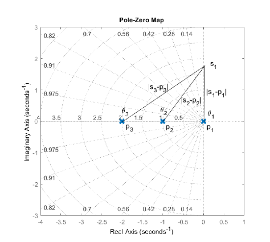
Let \(KGH(s)=\frac{K}{s(s+1)(s+2)}\); then, assuming that a point, \(s_1=j\sqrt{2}\), lies on the root locus, it satisfies the following conditions (Figure 5.1.6):

Magnitude condition: \(\frac{K}{|j\sqrt{2}|\,|1+j\sqrt{2}|\,|2+j\sqrt{2}|}=1\)

Angle condition: \(-\angle(j\sqrt{2})-\angle(1+j\sqrt{2})-\angle(2+j\sqrt{2})=-180^\circ\)

Figure \(\PageIndex{6}\): Displacements and angles from OL poles to a point on the RL.

Controller Design

The magnitude condition, \(\left|KGH(s_{1} )\right|=1\), can be solved for the static controller gain, \(K\), to get: \(K=\frac{\left|s_{1} -p_{1} \right|\ldots |s_{1} -p_{n} |}{\left|s_{1} -z_{1} \right|\ldots \left|s_{1} -z_{m} \right|}\).

Further, let \(\theta _{z_{i} } ,\theta _{p_{i} }\) denote the angles from the open-loop zeros and poles to the point \(s_{1}\); then, the angle condition states that: \(\sum \theta _{z_{i} } -\sum \theta _{p_{i} } =\pm 180^{\circ }\) (for \(K>0\)). Alternatively, \(\sum \theta _{z_{i} } -\sum \theta _{p_{i} } =0^{\circ }\) (for \(K<0\)).

The angle condition can be used to add poles and zeros to the feedback loop, i.e., design a dynamic controller that would force an RL branch to pass through a desired closed-loop root location.