6.0: Prelude to Compensator Design with Frequency Response Methods

Last updated
Save as PDF

Page ID: 24459

\( \newcommand{\vecs}[1]{\overset { \scriptstyle \rightharpoonup} {\mathbf{#1}} } \) \( \newcommand{\vecd}[1]{\overset{-\!-\!\rightharpoonup}{\vphantom{a}\smash {#1}}} \)\(\newcommand{\id}{\mathrm{id}}\) \( \newcommand{\Span}{\mathrm{span}}\) \( \newcommand{\kernel}{\mathrm{null}\,}\) \( \newcommand{\range}{\mathrm{range}\,}\) \( \newcommand{\RealPart}{\mathrm{Re}}\) \( \newcommand{\ImaginaryPart}{\mathrm{Im}}\) \( \newcommand{\Argument}{\mathrm{Arg}}\) \( \newcommand{\norm}[1]{\| #1 \|}\) \( \newcommand{\inner}[2]{\langle #1, #2 \rangle}\) \( \newcommand{\Span}{\mathrm{span}}\) \(\newcommand{\id}{\mathrm{id}}\) \( \newcommand{\Span}{\mathrm{span}}\) \( \newcommand{\kernel}{\mathrm{null}\,}\) \( \newcommand{\range}{\mathrm{range}\,}\) \( \newcommand{\RealPart}{\mathrm{Re}}\) \( \newcommand{\ImaginaryPart}{\mathrm{Im}}\) \( \newcommand{\Argument}{\mathrm{Arg}}\) \( \newcommand{\norm}[1]{\| #1 \|}\) \( \newcommand{\inner}[2]{\langle #1, #2 \rangle}\) \( \newcommand{\Span}{\mathrm{span}}\)\(\newcommand{\AA}{\unicode[.8,0]{x212B}}\)

Frequency response methods for designing compensators for feedback control systems predate the root locus and the time-domain (state variable) methods. They have been used effectively for designing amplifiers and filters in the case of electrical networks, and vibration analysis in the case of mechanical systems.

Control systems design using the frequency response method requires knowledge of \(KGH(j\omega )\). Strictly speaking, the knowledge of the plant transfer function \(G(s)\) is not needed. In the absence of a mathematical model, the plant transfer function can be identified from empirical measurements of the frequency response, \(G(j\omega )\).

The frequency response of a system can be graphed in multiple ways. The two most common representations are: [GrindEQ__1_] the Bode plot and [GrindEQ__2_] the Nyquist or Polar plot. The closed-loop frequency response may be visualized on the Nichol’s chart.

The frequency response design seeks to impart a certain degree of relative stability, measured by gain and phase margins, to the feedback control loop. The closed-loop system stability is alternatively ascertained by using the celebrated Nyquist criterion.

The peak gain in the closed-loop frequency response is a measure of the relative stability; the higher the peak the lower the relative stability. The crossover frequency on Bode magnitude plot and bandwidth on the closed-loop frequency response define measures of speed of response in the time-domain.

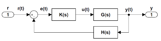
We consider standard feedback control system configuration (Figure 6.1) that includes a plant \(G(s)\), a sensor \(H(s)\), and a controller \(K(s)\). Unless stated otherwise, unity-gain feedback (\(H\left(s\right)=1\)) is assumed.

Figure \(\PageIndex{1}\): Copy and Paste Caption here. (Copyright; author via source)

In the following, we first review the plotting of frequency response and the associated performance metrics. Later, we will discuss the frequency response modification through adding phase-lead, phase-lag, lead–lag, PD, PI, and PID compensators to the control loop.