7.7: Root Locus Design of Digital Controllers

Digital Controller Design

The root locus technique (Chapter 5) employs the open-loop transfer function, \(KGH(s)\), to describe the locus of the roots of the closed-loop characteristic polynomial: \(\mathit{\Delta}\left(s\right)=1+KGH(s)\), with variation in the controller gain, \(K\).

The \(z\)-plane root locus similarly describes the locus of the roots of closed-loop pulse characteristic polynomial, \(\Delta (z)=1+KG(z)\), as controller gain \(K\) is varied. A suitable value of \(K\) can then be selected form the RL plot.

To ensure closed-loop stability, the closed-loop roots should be confined to inside the unit circle.

In the MATLAB Control Systems Toolbox, ‘rlocus’ command is used to plot both the \(s\)-plane and \(z\)-plane root loci. The RL design of digital controller is described below.

Design for a Desired Damping Ratio 

Assuming that the controller design specifications include a desired damping ratio, \(\zeta ,\) of the closed-loop poles, we consider the \(z\)-plane root locus design based on the \(\zeta\) requirement.

For a prototype second-order transfer function: \(T(s)=\frac{\omega _{n}^{2} }{s^{2} +2\zeta \omega _{n} s+\omega _{n}^{2} }\), the constant \(\zeta\) lines are defined by: \(\frac{\sigma }{\omega } =\mp \frac{\zeta }{\sqrt{1-\zeta ^{2} } }\). The constant \(\zeta\) lines in the z-plane are obtained by: \(z=e^{Ts} =e^{\sigma T} e^{\pm j\omega T}\), where \(\sigma =\mp \frac{\zeta }{\sqrt{1-\zeta ^{2} } } \omega\) and \(\omega T\) ranges from \(0\) to \(\pi\).

In the MATLAB Control Systems Toolbox, the ‘grid’ command displays the constant \(\zeta\) lines in the complex \(z\)-plane. The grid command additionally displays constant frequency \((\omega _{n} )\) contours that are helpful in selecting a suitable sampling time \((T)\) given the natural frequency of the model. The desired region in the \(z\)-plane for closed-loop root locations may be specified as: \(0.1\pi \le \omega _{n} T\le 0.5\pi ,\; \, \, \zeta \ge 0.6\), which assumes a sampling frequency between \(2\ and10\) times the natural frequency of the analog system.

Example \(\PageIndex{1}\)

Let \(G(s)=\frac{1}{s(s+1)}\), \(T=0.2\rm s\); then, we have: \(G(z)=\frac{0.0187z+0.0175}{(z-1)(z-0.819)}\). Assume that the design specifications call for \(\zeta =0.7\).

The closed-loop pulse characteristic polynomial is obtained as: \(\Delta (z)=z^{2} +(0.0187\, K-1.819)z+0.0175\, K+0.819.\)

The \(z\)-plane root locus is plotted using MATLAB 'rlocus' command and is shown in Fig. 7.7.1. From the z-plane RL plot (Figure 7.7.1), we can choose, e.g., \(K=0.46\), to have \(\zeta =0.7\) for the closed-loop roots.

Figure \(\PageIndex{1}\): Root locus design in the z-plane.

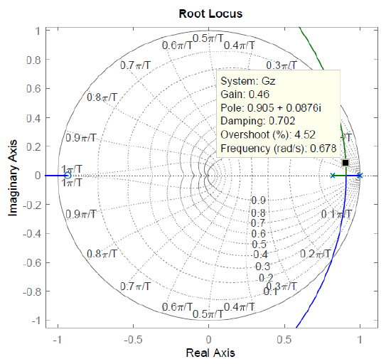
The resulting pulse characteristic polynomial is: \(\Delta (z)=z^{2} -1.81z+0.827,\) with closed-loop roots located at: \(z=0.9\pm j0.09.\) The use of MALTAB ‘damp’ command shows a damping ratio of \(\zeta =0.7\) with a natural frequency \(\omega _{n} =0.68\, \, {\rm rad/s}\).

For comparison, the continuous-time system has a characteristic polynomial: \(\Delta (s)=s^{2} +s+K,\); for \(K=0.46\), the closed-loop roots are located at \(s=0.5\pm j0.46\)with \(\zeta =0.74\) with \(\omega _{n} =0.68\, \, {\rm rad/s}\).

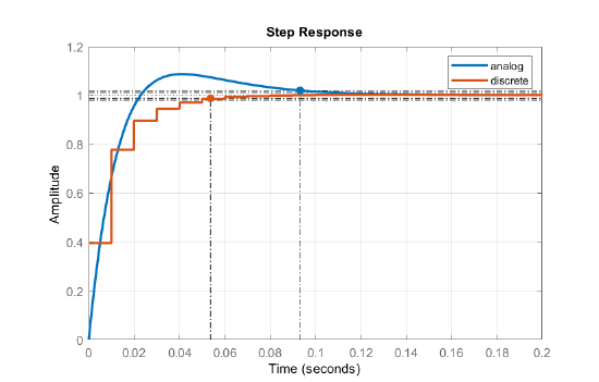
The step responses of analog and discrete systems are compared in Figure 7.7.2. 

 

Figure \(\PageIndex{2}\): Step response of the closed-loop continuous-time and sampled-data systems.

Design for Settling Time and Damping Ratio 

The settling time and the damping ratio of the dominant closed-loop roots in the \(z\)-plane are related as: \(re^{\pm j\theta } =e^{-\zeta \omega _{n} T} e^{\pm j\omega _ d T} ,\; \; \omega _ d =\omega _{n} \sqrt{1-\zeta ^{2} } .\)

By separating into real and imaginary part gives two equations: \(\ln r\; =-\zeta \omega _{n} T\) and \(\theta =\omega _{d} T\), which can be solved to obtain:

\[\zeta =-\ln r/\sqrt{\ln ^{2} r\; +\theta ^{2} } \nonumber \]

\[\omega _{n} =\sqrt{\ln ^{2} r\; +\theta ^{2} } /T \nonumber \]

\[\tau =\frac{1}{\zeta \omega _{n} } =-\frac{T}{\ln r\; } . \nonumber \]

Example \(\PageIndex{2}\)

Let \(G(z)=\frac{0.0187z+0.0175}{(z-1)(z-0.819)}\). The closed-loop pulse characteristic polynomial is obtained as: \(\Delta (z)=z^{2} +(0.0187\, K-1.819)z+0.0175\, K+0.819.\)

For \(\zeta =0.7\), the \(z\)-plane closed-loop roots are located at: \(z=0.905\pm j0.0875=0.91\; e^{\pm j0.096}\). Then, from the above relations, we obtain: \(\zeta =0.7,\; \omega _{n} =0.74,\; \tau =2.1\; {\rm s,\; }t_\rm s =4.6\, \tau =9.5\, \rm s.\)

A Comparison of Analog and Digital Controllers

The following example compares the root locus design of analog and digital controllers in the case of a DC motor model.

Example \(\PageIndex{3}\)

A DC motor model is described as: \(G\left(s\right)=\frac{500}{s^2+110s+1025}\); the design specifications are for the motor step response to have: \(OS\le 10\%\ (\zeta \ge 0.59),\ \ t_s\le 100ms,\ \ e{\left(\infty \right)|}_{step}=0.\)

The sampling time is selected as: \(T=0.01s\); then, from the MATLAB ‘c2d’ command, the motor pulse transfer function is obtained as:\(\ G\left(z\right)=\frac{0.0178z+0.0123}{z^2-1.27z+0.333}\).

In order to obtain zero steady-state error, we may choose a PI controller, where the controller zero approximately cancels a plant pole, i.e., let \(K\left(s\right)=\frac{K\left(s+10\right)}{s}\).

A comparable PI controller for the sampled-data system is obtained by using the transformation: \(z=e^{Ts}\), and is given as: \(K\left(z\right)=\frac{K\left(z-0.905\right)}{z-1}\).

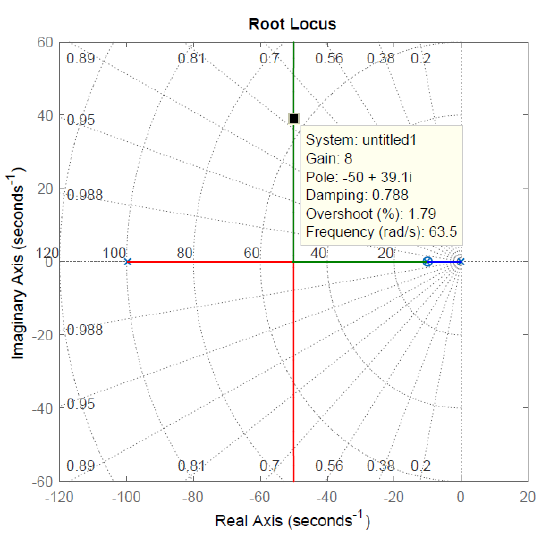
The \(s\)-plane and \(z\)-plane root locus plots are shown in Figure 7.7.3. From the plots, we may choose, e.g., \(K=8\) for the closed-loop system to achieve a time constant: \(\tau \cong 25ms\).

Figure \(\PageIndex{3}\): Root locus plot for the DC motor model: analog system design (left); sampled-data system design (right).

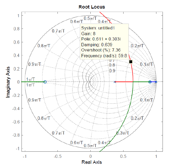
For \(K=8\), the resulting closed-loop transfer functions for analog and discrete system are obtained as:

Analog: \(T\left(s\right)=\frac{4000\left(s+10\right)}{s^3+110s^2+5025s+40,000}\)

Discrete: \(T\left(z\right)=\frac{0.14z^2-0.03z-0.089}{z^3-2.13z^2+1.57z-0.42}\)

The use of the MATLAB ‘damp’ command shows a damping of \(\zeta =0.79\) for the analog system and a damping of \(\zeta =0.68\) for the digital system.

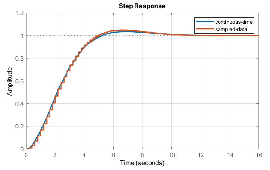
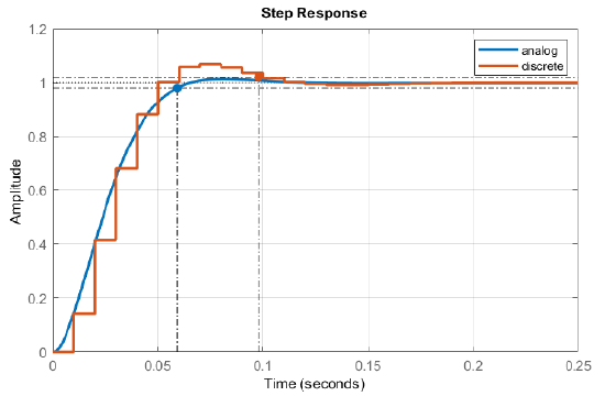
The step responses of the analog and discrete systems are compared in Figure 7.7.4. As seen from the figure, both analog and discrete systems meet the settling time and overshoot requirements.

Figure \(\PageIndex{4}\): Step response of the DC motor for the analog and discrete PI controller design.

MATLAB Tuned PID Controller Design 

The MATLAB Control Systems Toolbox provide ‘pidtune’ command that can be used with both analog and discrete system models. The tuned PID controller design in the case of a DC motor is explored in the next example.

Example \(\PageIndex{4}\)

Let \(G\left(s\right)=\frac{500}{s^2+110s+1025}\); the design specifications are for the motor step response to have: \(OS\le 10\%\ (\zeta \ge 0.59),\ \ t_s\le 100ms,\ \ e{\left(\infty \right)|}_{step}=0.\)

Let \(T=0.01s\); from the MATLAB ‘c2d’ command, the motor pulse transfer function is obtained as:\(\ G\left(z\right)=\frac{0.0178z+0.0123}{z^2-1.27z+0.333}\).

By using the MATLAB ‘pidtune’ command, an analog PID controller for the DC motor model with a crossover frequency of \(100rad/s\) is obtained as: \(K\left(s\right)=25.1+0.189s+\frac{567}{s}\).

The ‘pidtune’ command is used to design a similar PID controller for the discrete model. The result is: \(K\left(z\right)=23.4+0.368\left(\frac{z-1}{T}\right)+202\left(\frac{T}{z-1}\right)\).

The unit-step responses of the closed-loop systems for the analog and discrete models are compared in Figure 7.7.5. Both controller achieve a settling time \(t_s<0.1s\) with no steady-state error. However, in this case, the tuned digital PID controller has a lower settling time.

Figure \(\PageIndex{5}\): Step response of the DC motor for the analog and discrete PID controller design.