8.1: State Variable Models

The State Equations

The state variable model of a dynamic system comprises first-order ODEs that describe time derivatives of a set of state variables. The number of state variables represents the order of the system, which is assumed to match the degree of the denominator polynomial in its transfer function description.

The natural variables associated with the energy storing elements are commonly used as state variables, though alternate variables can be selected. The natural variables include, for example, capacitor voltage and inductor current in the electrical networks, and position and velocity of the inertial mass in the mechanical systems.

Let \({\bf x}(t)\) describe a vector of state variables, \(u(t)\) describe a scalar input, and \(y(t)\) describe a scalar output; then the state variable model of a linear time-invariant (LTI) single-input single-output (SISO) system is written in its generic form as:

\[\dot{\bf x}(t)={\bf Ax}(t)+{\bf b}u(t) \nonumber \]

\[y(t)={\bf c}^{T} {\bf x}(t)+du(t) \nonumber \]

In the above, \(\bf A\) is an \(n\times n\) matrix, \(\bf b\) is a column vector that distributes the inputs, \({\bf c}^{T}\) is a row vector that combines the state variables to form the output, and \( d\) is a scalar feedforward term contributing to the output.

The state variable model of a multi-input multi-output (MIMO) system with \(m\) inputs and \(p\) outputs is described by the state and output equations given as:

\[\dot{\bf x}(t)={\bf Ax}(t)+{\bf Bu}(t) \nonumber \]

\[{\bf y}(t)={\bf C}^{T} {\bf x}(t)+{\bf Du}(t) \nonumber \]

In the above, the variable dimensions are: \({\bf x}\in {\bf R}^n,\ {\bf u}\in {\bf R}^m,\ \ \rm and\ {\bf y}\in {\bf R}^p\); the matrices have the following dimensions:\({\bf A}\in {\bf R}^{n\times n},\ {\bf B}\in {\bf R}^{n\times m},\ {\bf C}\in {\bf R}^{p\times n},\ {\rm and}\ {\bf D}\in {\bf R}^{p\times m}\).

In the following, we restrict our attention to models of SISO systems. Unless noted otherwise,  \(d=0\) is assumed, which corresponds to a strictly proper transfer function description of the system.

Solution to the State Equations

In order to explore a time-domain solution to the state equations, we begin with a scalar differential equation:

\[\dot{x}(t)=ax(t)+bu(t). \nonumber \]

Using an integrating factor, \(e^{-at}\), the equation is written as total differential:

\[\frac {d}{ dt} (e^{-at} x(t))=e^{-at} bu(t) \nonumber \]

Next, assuming an initial conditions: \(x\left(0\right)=x_0\), we integrate from \(\tau =0\) to \(\tau =t\) to obtain:

\[e^{-at} x(t)-x_{0} =\int _{0}^{\tau } e^{-a\tau } bu(\tau ) d\tau \nonumber \]

Hence, the solution to the scalar ODE in terms of \(x(t)\) is obtained as:

\[x(t)=e^{at} x_{0} +\int _{0}^{\tau } e^{a(t-\tau )} bu(\tau ) d\tau \nonumber \]

Further, the solution to homogeneous equation: \(\dot{x}\left(t\right)=ax\left(t\right)\) is given as: \(x\left(t\right)=e^{at}x_0.\)

Next, we explore the possibility to generalize this solution to the matrix case. For this purpose, we define a matrix exponential function as:

\[e^{{\bf A}t} =\sum _{i=0}^{\infty } \frac{{\bf A}^{i} t^{i} }{i!} ={\bf I}+{\bf A}t+\ldots \nonumber \]

The infinite series converges in the case of systems that are well-behaved. Further, the matrix exponential obeys the matrix differential equation:

\[\frac{d}{dt} \left(e^{{\bf A}t} \right)={\bf A}e^{{\bf A}t} =e^{{\bf A}t} {\bf A} \nonumber \]

Using the matrix exponential, the solution to the matrix differential equation, \(\dot{\bf x}(t)={\bf Ax}(t)+{\bf b}u(t)\), is written as:

\[{\bf x}(t)=e^{{\bf A}t} {\bf x}_{0} +\int _{0}^{\tau } e^{{\bf A}(t-\tau )} {\bf b}u(\tau ) d\tau \nonumber \]

The above solution has two parts: the first term describes the system response to initial conditions \({\bf x}_{0}\), while the second term describes the system response to an input, \(u(t)\).

Laplace Transform Solution

Consider the state equation:

\[ \dot{\bf x}(t)={\bf Ax}(t)+{\bf b}u(t) , {\bf x}\left(0\right)={\bf x}_0; \nonumber \]

Apply the Laplace transform to obtain:

\[s{\bf x}(s)-{\bf x}_{0} ={\bf Ax}(s)+{\bf b}u(s). \nonumber \]

The state variable vector is solved as:

\[{\bf x}(s)=(s{\bf I}-{\bf A})^{-1} {\bf x}_{0} +(s{\bf I-A})^{-1} {\bf b}u(s), \nonumber \]

where \({\bf I}\) denote an \(n\times n\) identity matrix. 

The \(n\times n\) matrix \((s{\bf I-A})\) is called the characteristic matrix of \({\bf A}\).

Its determinant defines the characteristic polynomial of \({\bf A}\), i.e., \(\Delta (s)=|s{\bf I}-{\bf A}|\).

The roots of the characteristic polynomial are the eigenvalues of \({\bf A}\).

The \(n\times n\) matrix \((s{\bf I}-{\bf A})^{-1}\) is called the resolvent matrix of \({\bf A}\). The resolvent of \({\bf A}\) can be computed as an infinite series:

\[(s{\bf I}-{\bf A})^{-1} =s^{-1} ({\bf I}+s^{-1} {\bf A}+\ldots ) \nonumber \]

By comparing the Laplace transform solution with the time-domain solution, we arrive at the following relations:

\[{\rm\mathcal L}[e^{{\bf A}t} ]=(s{\bf I}-{\bf A})^{-1} \nonumber \]

\[ {\rm {\mathcal L}}\left[\int _{0}^{\tau } e^{{\bf A}(t-\tau )} {\bf b}u(\tau ) d\tau \right]=(s{\bf I}-{\bf A})^{-1} {\bf b}u(s) \nonumber \]

The first equation above can be used to compute the matrix exponential:

\[e^{{\bf A}t} ={\rm L}^{\rm -1} \left[(s{\bf I}-{\bf A})^{-1} \right] \nonumber \]

The second equation is used to solve for the output response when initial conditions are zero:

\[y(s)={\bf c}^{T} (s{\bf I}-{\bf A})^{-1} {\bf b}u(s) \nonumber \]

The State-Transition Matrix

Consider the homogenous system of equations: \(\dot{\bf x}(t)={\bf Ax}(t)\, \, {\rm and}\, \, {\bf x}(0)={\bf x}_{0}\).

The solution to the homogenous state equation is given as: \({\bf x}(t)=e^{{\bf A}t} {\bf x}_{0}\).

The matrix exponential \(e^{{\bf A}t}\) that relates \({\bf x}_{0}\) to \({\bf x}(t)\) is termed as the state-transition matrix. The state-transition matrix contains the natural modes of system response. 

Transfer Function

The output response of the state variable model defines the transfer function: \(y(s)=G(s)u(s)\), where

\[G(s)={\bf c}^{T} (s{\bf I}-{\bf A})^{-1} {\bf b}= {\bf c}^{T}\frac{\rm adj (s{\bf I}-{\bf A})}{\det (s{\bf I}-{\bf A})}{\bf b} \nonumber \]

In the case of a MIMO system, \(G\left(s\right)\) represents a \(p\times m\) transfer matrix, given as:

\[G(s)={\bf C}(s{\bf I}-{\bf A})^{-1} {\bf B+D} \nonumber \]

Alternatively, the transfer matrix of a MIMO system can be obtained as:

\[G(s)=\frac{\rm det \left[\begin{array}{cc} s{\bf I-A} & -{\bf B} \\ {\bf C} & {\bf D} \end{array}\right]}{\det (s{\bf I-A})} \nonumber \]

Assuming no pole-zero cancelations in \(G\left(s\right)\), the characteristic polynomial matches the denominator polynomial.In the event of pole-zero cancelations, the order of the denominator polynomial, \(d\left(s\right)\), is less than \(n\), i.e., the zeros of \(d\left(s\right)\) form a subset of the eigenvalues of \({\bf A}\).

Example \(\PageIndex{1}\)

Consider the mass–spring–damper model (Example 1.9.2), where mass position, \(x(t)\), and velocity, \(v(t)=\dot{x}(t)\) are selected as state variables; then, the state output equations are given as:

\[\frac{\rm d}{\rm dt} \left[\begin{array}{c} {x} \\ {v} \end{array}\right]=\left[\begin{array}{cc} {0} & {1} \\ -\frac{k}{m} & -\frac{b}{m} \end{array}\right] \left[\begin{array}{c} {x} \\ {v} \end{array}\right]+\left[\begin{array}{c} {0} \\ \frac{1}{m} \end{array}\right]f, \;\;x=\left[\begin{array}{cc} {1} & {0} \end{array}\right] \left[\begin{array}{c} {x} \\ {v} \end{array}\right] \nonumber \]

The characteristic matrix of the model is given as: \(s{\bf I-A}=\left[\begin{array}{cc} {s} & {-1} \\ {\frac{k}{m} } & {s+\frac{b}{m} } \end{array}\right]\).

The resolvent of \({\bf A}\) is computed as: \((s{\bf I-A})^{-1} =\frac{1}{\Delta (s)} \left[\begin{array}{cc} {s+b/m} & {1} \\ {-k/m} & {s} \end{array}\right];\; \; \Delta (s)=s^{2} +\frac{b}{m} s+\frac{k}{m}\).

The transfer function of the model is computed as: \[G(s)=\frac{1}{\Delta(s)}=\left[\begin{array}{cc} {0} & {1} \end{array}\right] \left[\begin{array}{cc} {s+b/m} & {1} \\ {-k/m} & {s} \end{array}\right] \left[\begin{array}{c} 1\\ \frac{1}{m} \end{array}\right]=\frac{1}{ms^2 +bs+k} \nonumber \]

Example \(\PageIndex{2}\)

Consider the model of a DC motor (Example 1.9.3), where armature current, \(i_a(t)\), and motor speed, \(\omega (t)\), are selected as state variables; the state and output equations of the DC motor are given as:

\[\frac {d}{ dt} \left[\begin{array}{c} {i_a} \\ {\omega} \end{array}\right] = \left[\begin{array}{cc} {-R/L} & {-k_b /L} \\ {k_{t} /J} & {-b/J} \end{array}\right] \left[\begin{array}{c} {i_a} \\ {\omega} \end{array}\right]+\left[\begin{array}{c} {1/L} \\ {0} \end{array}\right] V_{a} ,\;\; \omega =\left[\begin{array}{cc} {0} & {1} \end{array}\right]\left[\begin{array}{c} {i_a } \\ {\omega } \end{array}\right] \nonumber \]

Assume that the following parameter values be assumed:\(R=1\Omega ,\; L=1\; mH,\; \; J=0.01\; kg \cdot m^2 ,\; b=0.1\; \frac{{ N}\cdot s}{rad} ,\; k_t = k_b =0.05\). Then, the state variable model of the motor is given as:

\[\frac {d}{ dt} \left[\begin{array}{c} {i_a } \\ {\omega } \end{array}\right]=\left[\begin{array}{cc} {-100} & {-5} \\ {5} & {-10} \end{array}\right]\left[\begin{array}{c} {i_a } \\ {\omega } \end{array}\right]+\left[\begin{array}{c} {100} \\ {0} \end{array}\right] V_{ a}, \;\; \omega =\left[\begin{array}{cc} {0} & {1} \end{array}\right]\left[\begin{array}{c} {i_a } \\ {\omega } \end{array}\right] \nonumber \]

The resolvent matrix and the motor transfer function is obtained as follows:

\[(s{\bf I-A})^{-1} =\frac{1}{\Delta (s)} \left[\begin{array}{cc} {s+10} & {-5} \\ {5} & {s+100} \end{array}\right];\; \; \Delta (s)=s^{2} +110s+1025 \nonumber \]

\[G(s)={\bf c}^{T} (s{\bf I-A})^{-1} {\bf b}=\frac{500}{s^{2} +110s+1025} \nonumber \]

Impulse Response

Consider the state equation:

\[\dot{\bf x}(t)={\bf Ax}(t)+{\bf b}u(t), \;\; y(t)={\bf c}^T {\bf x} \nonumber \]

For \({\bf x}_0={\bf 0}\), the input response of the system is obtained as:

\[y\left(s\right)=G\left(s\right)u\left(s\right)={\bf c}^T\left(s{\bf I-A}\right)^{-1}{\bf b}u(s) \nonumber \]

Let \(u\left(t\right)=\delta \left(t\right),\ \ u\left(s\right)=1\); then, the system response is given as:

\[y_{imp}\left(s\right)=G(s)={\bf c}^T\left(s{\bf I-A}\right)^{-1}{\bf b} \nonumber \]

The impulse response in the time-domain is obtained as:

\[g\left(t\right)={\rm \mathcal L}^{\rm -1} \left[G(s)\right]={\bf c}^Te^{{\bf A}t}{\bf b} \nonumber \]

In terms of the impulse response, the system output is given by the convolution integral:

\[y\left(t\right)=\int^t_0{g\left(t-\tau \right)u\left(\tau \right)d\tau } \nonumber \]

Step Response 

Let \(u\left(t\right)=1\left(t\right),\ \ u\left(s\right)=\frac{1}{s}\). Then, we have:

\[s{\bf x}\left(s\right)={\bf c}^T\left(s{\bf I-A}\right)^{-1}{\bf b} \nonumber \]

The unit-step response in time-domain is obtained as:

\[y_{step}\left(t\right)={\bf c}^T\left(\int^t_0{e^{{\bf A}\left(t-\tau \right)}d\tau }\right){\bf b} \nonumber \]

Alternatively, the step response represents the integral of the impulse response:

\[y_{step}\left(t\right)=\int^t_0{g\left(t-\tau \right)d\tau } \nonumber \]

Exercise \(\PageIndex{3}\)

The state and output equations for the model of a dc motor are:

\[\frac{\rm d}{\rm dt} \left[\begin{array}{c} {i_a } \\ {\omega } \end{array}\right]=\left[\begin{array}{cc} {-100} & {-5} \\ {5} & {-10} \end{array}\right] \left[\begin{array}{c} {i_a } \\ {\omega } \end{array}\right]+\left[\begin{array}{c} {100} \\ {0} \end{array}\right] V_a, \omega =\left[\begin{array}{cc} {0} & {1} \end{array}\right]\left[\begin{array}{c} {i_a } \\ {\omega } \end{array}\right] \nonumber \]

The state-transition matrix for the dc motor model is obtained as:

\[e^{{\bf A}t} =\left[\begin{array}{cc} {1.003} & {0.056} \\ {-0.056} & {-0.003} \end{array}\right]e^{-99.72t} +\left[\begin{array}{cc} {-0.003} & {-0.056} \\ {0.056} & {1.0003} \end{array}\right]e^{-10.28t} \nonumber \]

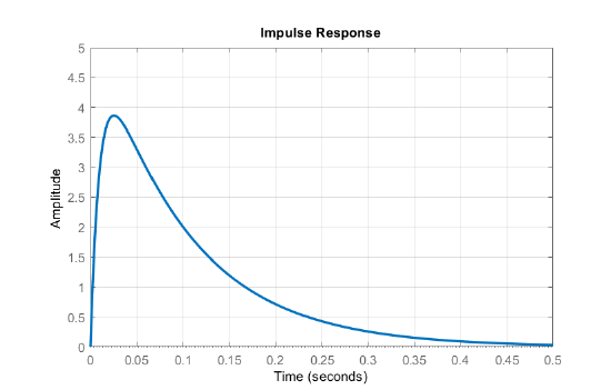
The impulse response of the DC motor is computed as:

\[g\left(t\right)={\bf c}^Te^{{\bf A}t}{\bf b}=5.6\left(e^{-99.7t}-e^{-10.3t}\right) \nonumber \]

where \(\left\{e^{-99.72t} ,\; e^{-10.28t} \right\}\) represent the system’s natural response modes that correspond to the electrical and mechanical time constants of the DC motor: \(\tau _{\rm e} \cong 0.01s,\; \tau _\rm m \cong 0.1\rm s\).

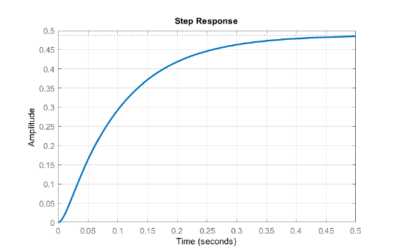
Assuming \(V_a\left(t\right)=u\left(t\right)\), the step response of the DC motor is computed as:

\[y\left(t\right)=\int^t_0{g\left(t-\tau \right)d\tau }=0.488+0.056e^{-99.7t}-0.544e^{-10.3t} \nonumber \]

The impulse and the step responses are plotted below (Figures 8.1.1).

Figure \(\PageIndex{1}\): The DC motor model: impulse response (left); step response (right).