8.3: State-Space Realization of Transfer Function Models
- Page ID
- 24426
\( \newcommand{\vecs}[1]{\overset { \scriptstyle \rightharpoonup} {\mathbf{#1}} } \)
\( \newcommand{\vecd}[1]{\overset{-\!-\!\rightharpoonup}{\vphantom{a}\smash {#1}}} \)
\( \newcommand{\dsum}{\displaystyle\sum\limits} \)
\( \newcommand{\dint}{\displaystyle\int\limits} \)
\( \newcommand{\dlim}{\displaystyle\lim\limits} \)
\( \newcommand{\id}{\mathrm{id}}\) \( \newcommand{\Span}{\mathrm{span}}\)
( \newcommand{\kernel}{\mathrm{null}\,}\) \( \newcommand{\range}{\mathrm{range}\,}\)
\( \newcommand{\RealPart}{\mathrm{Re}}\) \( \newcommand{\ImaginaryPart}{\mathrm{Im}}\)
\( \newcommand{\Argument}{\mathrm{Arg}}\) \( \newcommand{\norm}[1]{\| #1 \|}\)
\( \newcommand{\inner}[2]{\langle #1, #2 \rangle}\)
\( \newcommand{\Span}{\mathrm{span}}\)
\( \newcommand{\id}{\mathrm{id}}\)
\( \newcommand{\Span}{\mathrm{span}}\)
\( \newcommand{\kernel}{\mathrm{null}\,}\)
\( \newcommand{\range}{\mathrm{range}\,}\)
\( \newcommand{\RealPart}{\mathrm{Re}}\)
\( \newcommand{\ImaginaryPart}{\mathrm{Im}}\)
\( \newcommand{\Argument}{\mathrm{Arg}}\)
\( \newcommand{\norm}[1]{\| #1 \|}\)
\( \newcommand{\inner}[2]{\langle #1, #2 \rangle}\)
\( \newcommand{\Span}{\mathrm{span}}\) \( \newcommand{\AA}{\unicode[.8,0]{x212B}}\)
\( \newcommand{\vectorA}[1]{\vec{#1}} % arrow\)
\( \newcommand{\vectorAt}[1]{\vec{\text{#1}}} % arrow\)
\( \newcommand{\vectorB}[1]{\overset { \scriptstyle \rightharpoonup} {\mathbf{#1}} } \)
\( \newcommand{\vectorC}[1]{\textbf{#1}} \)
\( \newcommand{\vectorD}[1]{\overrightarrow{#1}} \)
\( \newcommand{\vectorDt}[1]{\overrightarrow{\text{#1}}} \)
\( \newcommand{\vectE}[1]{\overset{-\!-\!\rightharpoonup}{\vphantom{a}\smash{\mathbf {#1}}}} \)
\( \newcommand{\vecs}[1]{\overset { \scriptstyle \rightharpoonup} {\mathbf{#1}} } \)
\(\newcommand{\longvect}{\overrightarrow}\)
\( \newcommand{\vecd}[1]{\overset{-\!-\!\rightharpoonup}{\vphantom{a}\smash {#1}}} \)
\(\newcommand{\avec}{\mathbf a}\) \(\newcommand{\bvec}{\mathbf b}\) \(\newcommand{\cvec}{\mathbf c}\) \(\newcommand{\dvec}{\mathbf d}\) \(\newcommand{\dtil}{\widetilde{\mathbf d}}\) \(\newcommand{\evec}{\mathbf e}\) \(\newcommand{\fvec}{\mathbf f}\) \(\newcommand{\nvec}{\mathbf n}\) \(\newcommand{\pvec}{\mathbf p}\) \(\newcommand{\qvec}{\mathbf q}\) \(\newcommand{\svec}{\mathbf s}\) \(\newcommand{\tvec}{\mathbf t}\) \(\newcommand{\uvec}{\mathbf u}\) \(\newcommand{\vvec}{\mathbf v}\) \(\newcommand{\wvec}{\mathbf w}\) \(\newcommand{\xvec}{\mathbf x}\) \(\newcommand{\yvec}{\mathbf y}\) \(\newcommand{\zvec}{\mathbf z}\) \(\newcommand{\rvec}{\mathbf r}\) \(\newcommand{\mvec}{\mathbf m}\) \(\newcommand{\zerovec}{\mathbf 0}\) \(\newcommand{\onevec}{\mathbf 1}\) \(\newcommand{\real}{\mathbb R}\) \(\newcommand{\twovec}[2]{\left[\begin{array}{r}#1 \\ #2 \end{array}\right]}\) \(\newcommand{\ctwovec}[2]{\left[\begin{array}{c}#1 \\ #2 \end{array}\right]}\) \(\newcommand{\threevec}[3]{\left[\begin{array}{r}#1 \\ #2 \\ #3 \end{array}\right]}\) \(\newcommand{\cthreevec}[3]{\left[\begin{array}{c}#1 \\ #2 \\ #3 \end{array}\right]}\) \(\newcommand{\fourvec}[4]{\left[\begin{array}{r}#1 \\ #2 \\ #3 \\ #4 \end{array}\right]}\) \(\newcommand{\cfourvec}[4]{\left[\begin{array}{c}#1 \\ #2 \\ #3 \\ #4 \end{array}\right]}\) \(\newcommand{\fivevec}[5]{\left[\begin{array}{r}#1 \\ #2 \\ #3 \\ #4 \\ #5 \\ \end{array}\right]}\) \(\newcommand{\cfivevec}[5]{\left[\begin{array}{c}#1 \\ #2 \\ #3 \\ #4 \\ #5 \\ \end{array}\right]}\) \(\newcommand{\mattwo}[4]{\left[\begin{array}{rr}#1 \amp #2 \\ #3 \amp #4 \\ \end{array}\right]}\) \(\newcommand{\laspan}[1]{\text{Span}\{#1\}}\) \(\newcommand{\bcal}{\cal B}\) \(\newcommand{\ccal}{\cal C}\) \(\newcommand{\scal}{\cal S}\) \(\newcommand{\wcal}{\cal W}\) \(\newcommand{\ecal}{\cal E}\) \(\newcommand{\coords}[2]{\left\{#1\right\}_{#2}}\) \(\newcommand{\gray}[1]{\color{gray}{#1}}\) \(\newcommand{\lgray}[1]{\color{lightgray}{#1}}\) \(\newcommand{\rank}{\operatorname{rank}}\) \(\newcommand{\row}{\text{Row}}\) \(\newcommand{\col}{\text{Col}}\) \(\renewcommand{\row}{\text{Row}}\) \(\newcommand{\nul}{\text{Nul}}\) \(\newcommand{\var}{\text{Var}}\) \(\newcommand{\corr}{\text{corr}}\) \(\newcommand{\len}[1]{\left|#1\right|}\) \(\newcommand{\bbar}{\overline{\bvec}}\) \(\newcommand{\bhat}{\widehat{\bvec}}\) \(\newcommand{\bperp}{\bvec^\perp}\) \(\newcommand{\xhat}{\widehat{\xvec}}\) \(\newcommand{\vhat}{\widehat{\vvec}}\) \(\newcommand{\uhat}{\widehat{\uvec}}\) \(\newcommand{\what}{\widehat{\wvec}}\) \(\newcommand{\Sighat}{\widehat{\Sigma}}\) \(\newcommand{\lt}{<}\) \(\newcommand{\gt}{>}\) \(\newcommand{\amp}{&}\) \(\definecolor{fillinmathshade}{gray}{0.9}\)Simulation Diagrams
We consider the problem of realizing a given transfer function model as a state variable model. The realization process is facilitated by first drawing a simulation diagram for the system.
A simulation diagram realizes an ODE model into a block diagram representation using scalar gains, integrators, summing nodes, and feedback loops. Historically, such diagrams were used to simulate dynamic system models on analog computers.
Given a transfer function model, its two common realizations are described below.
Serial Realization
A serial chain of integrators can be used to realize the output of an ODE. To illustrate this idea, we consider a general second-order system model described as:
\[\frac{y\left(s\right)}{u\left(s\right)}=\frac{K}{s^2+2\zeta {\omega }_ns+{\omega }^2_n} \nonumber \]
The transfer function is converted into an ODE representation by cross multiplying followed by inverse Laplace transform to obtain:
\[\ddot{y}\left(t\right)+2\zeta {\omega }_n\dot{y}\left(t\right)+{\omega }^2_ny\left(t\right)=Ku\left(t\right) \nonumber \]
The above equation is rearranged to form the highest derivative as:
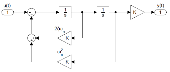
\[\ddot{y}\left(t\right)=-2\zeta {\omega }_n\dot{y}\left(t\right)-{\omega }^2_ny\left(t\right)+Ku\left(t\right) \nonumber \]
The simulation diagram first realizes the highest derivative using a summing node and then uses a series of integrators to obtain the lower order derivatives up to the output (Figure 8.3.1).

Parallel Realization
Consider a second-order transfer function with real roots expressed as: \[\frac{y\left(s\right)}{u\left(s\right)}=\frac{K}{s^2+\left(\sigma_1+\sigma_2\right)s+\sigma_1\sigma_2} \nonumber \]
The transfer function can be expanded using partial fractions expansion (PFE) to obtain: \[y(s)=\frac{K_1}{s+\sigma_1}u(s)+\frac{K_2}{s+\sigma_2}u(s) \nonumber \]
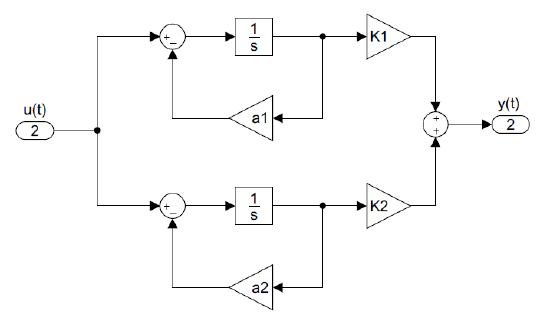
In parallel realization, the system output is expressed as: \(y\left(s\right)=y_1\left(s\right)+y_2\left(s\right)\); further, the two output components are formed by ODEs that share a common input, \(u\left(t\right)\): \[\sigma_i{\dot{y}}_i\left(t\right)+y_i\left(t\right)=K_iu\left(t\right),\ \ i=1,2 \nonumber \]
These ODEs are realized into a parallel simulation diagram (Figure 8.3.2).

Having drawn a simulation diagram, we designate the outputs of the integrators as state variables and express integrator inputs as first-order differential equations, referred as the state equations. A serial realization acquires a controller form structure; a parallel realization acquires a modal structure. These are discussed below.
Controller Form Realization
A controller form state variable structure results from a serial realization of the transfer function model. This is illustrated using a third-order transfer function model:
\[G(s)=\frac{b_{1} s^{2} +b_{2} s+b_{3} }{s^{3} +a_{1} s^{2} +a_{2} s+a_{3} } \nonumber \]
The above transfer function corresponds to the following ODE:
\[\stackrel{...}{y}(t)+a_{1} \ddot{y}(t)+a_{2} \dot{y}(t)+a_{3} y(t)=b_{1} \ddot{u}(t)+b_{2} \dot{u}(t)+b_{3} u(t) \nonumber \]
To remove the derivatives of the input from state variables, an auxiliary variable, \(v(t)\), is introduced to split the ODE as:
\[\stackrel{...}{v}(t)+a_{1} \ddot{v}(t)+a_{2} \dot{v}(t)+a_{3} v(t)=u(t) \nonumber \] \[y(t)=b_{1} \ddot{v}(t)+b_{2} \dot{v}(t)+b_{3} v(t) \nonumber \]
The highest derivative term in the first ODE is realized using a summing node:
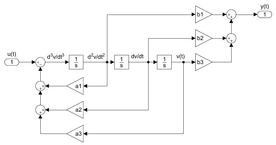
\[\stackrel{...}{v}(t)=-a_{1} \ddot{v}(t)-a_{2} \dot{v}(t)-a_{3} v(t)+u(t) \nonumber \]
The lower order derivative terms, \(\ddot{v}(t)\) and \(\dot{v}(t)\), and the output, \(v\left(t\right)\), are realized using integrators.
The second ODE can be realized by summing the outputs of the integrators using coefficients as weights (Figure 8.3.3).

Next, the state variables are designated as: \(x_{1} (t)=v(t),\; x_{2} (t)=\dot{v}(t),\; x_{3} (t)=\ddot{v}(t)\).
The resulting state equations are: \[{\dot{x}}_1=x_2, \\ {\dot{x}}_2=x_3, \\ {\dot{x}}_3=-a_3x_1-a_2x_2-a_3x_3+u \nonumber \]
The output equation is given as: \[y=b_1x_1+b_2x_2+b_3x_3 \nonumber \]
In vector–matrix form, the state variable model is given as:
\[\frac{d}{dt} \left[\begin{array}{c} {x_{1} } \\ {x_{2} } \\ {x_{3} } \end{array}\right]=\left[\begin{array}{ccc} {0} & {1} & {0} \\ {0} & {0} & {1} \\ {-a_{3} } & {-a_{2} } & {-a_{1} } \end{array}\right]\left[\begin{array}{c} {x_{1} } \\ {x_{2} } \\ {x_{3} } \end{array}\right]+\left[\begin{array}{c} {0} \\ {0} \\ {1} \end{array}\right]u,\;\; y=\left[\begin{array}{ccc} {b_{1} } & {b_{2} } & {b_{3} } \end{array}\right]\left[\begin{array}{c} {x_{1} } \\ {x_{2} } \\ {x_{3} } \end{array}\right] \nonumber \]
Generalization to \(n\) Variables
The controller form realization is generalized to \(n\) variables as follows: let \(G\left(s\right)=\frac{n\left(s\right)}{d\left(s\right)}\), where \(d(s)=s^{n} +a_{1} s^{n-1} +\ldots +a_{n-1} s+a_{n} \) represents the denominator polynomial.
By selecting the output variable and its derivatives: \(y(t),\dot{y}(t),\ldots ,y^{(n-1)} (t)\), as state variables, we obtain the following controller form structure:
\[A=\left[\begin{array}{cc} {\begin{array}{cc} {0\; \; \; \; \; \; \; } & {1} \\ {0\; \; \; \; \; \; \; } & {0} \end{array}} & {\begin{array}{cc} {0\; \; \; } & {\ldots } \\ {1\; \; \; } & {\ldots } \end{array}} \\ {\begin{array}{cc} {\vdots } & {\vdots } \\ {-a_{n} } & {-a_{n-1} } \end{array}} & {\begin{array}{cc} {\ddots } & {1} \\ {\ldots } & {-a_{1} } \end{array}} \end{array}\right],\; \; b=\left[\begin{array}{c} {\begin{array}{c} {0} \\ {0} \end{array}} \\ {\begin{array}{c} {\vdots } \\ {1} \end{array}} \end{array}\right] \nonumber \]
Let \(n\left(s\right)=b_0s^m+b_1s^{m-1}+\dots +b_m\) represent the numerator polynomial, where \(m=n-1\) is assumed; then, the output matrix is formed as: \[c^T=\left[b_0\quad b_1\quad \dots \quad b_m\right] \nonumber \]
In the above controller form structure, the coefficients of the characteristic polynomial appear in reverse order in the last row of the system matrix, whereas the output matrix contains the coefficients of the numerator polynomial.
Hence, given a proper transfer function, \(G(s)\), the controller form can be written by inspection as shown in the following example.
A mass–spring–damper system is described by transfer function model: \(G\left(s\right)=\frac{y\left(s\right)}{u(s)}=\frac{1}{s^2+2s+2}\).
Its controller form state variable model is given as:
\[\frac{\rm d}{\rm dt} \left[\begin{array}{c} {x_{1} } \\ {x_{2} } \end{array}\right]=\left[\begin{array}{cc} {0} & {1} \\ {-2} & {-2} \end{array}\right]\, \left[\begin{array}{c} {x_{1} } \\ {x_{2} } \end{array}\right]+\left[\begin{array}{c} {0} \\ {1} \end{array}\right]\, u,\, \, \, y=\left[\begin{array}{cc} {1} & {0} \end{array}\right]\, \left[\begin{array}{c} {x_{1} } \\ {x_{2} } \end{array}\right] \nonumber \]
Alternate Controller Form Structure
The integrator outputs in the simulation diagram can be alternatively numbered left to right; this reorders the state variables whereby the coefficients of the characteristic polynomial appear in the first row of the matrix. For the third-order model presented in Fig. 8.3.3, the resulting equations are given as:
\[{\dot{x}}_3=-a_1 x_1 - a_2 x_2 - a_3 x_3+u,\\ {\dot{x}}_2=x_1 \\ {\dot{x}}_3=x_2 \nonumber \]
The alternate controller form is obtained by using 'ss' command after defining a transfer function in the MATLAB Control Systems Toolbox.
A mass–spring–damper system is described by the following transfer function: \(G\left(s\right)=\frac{y\left(s\right)}{u(s)}=\frac{1}{s^2+2s+2}\). The controller form state variable model is given as:
\[\frac{\rm d}{\rm dt} \left[\begin{array}{c} {x_{1} } \\ {x_{2} } \end{array}\right]=\left[\begin{array}{cc} {-2} & {-2} \\ {1} & {0} \end{array}\right]\, \left[\begin{array}{c} {x_{1} } \\ {x_{2} } \end{array}\right]+\left[\begin{array}{c} {1} \\ {0} \end{array}\right]\, u,\, \, \, y=\left[\begin{array}{cc} {0} & {1} \end{array}\right]\, \left[\begin{array}{c} {x_{1} } \\ {x_{2} } \end{array}\right] \nonumber \]
The state variables are numbered in reverse order. Hence, \(x_1\) represents the velocity and \(x_2\) the position of the inertial mass.
Dual (Observer Form) Realization
Assume that a state variable realization of the transfer function model is given as:
\[\dot{x}(t)=Ax(t)+bu(t), \;\;y(t)=c^{T} x(t) \nonumber \]
Its dual realization is defined by the following state variable model:
\[\dot{z}(t)=A^{T} z(t)+cu(t),\;\; y(t)=b^{T} z(t) \nonumber \]
Both the original and the dual models share the same scalar transfer function, i.e.,
\[G(s)=c^{T} (sI-A)^{-1} b=b^T{\left(sI-A^T\right)}^{-1}c=G^T\left(s\right) \nonumber \]
When the original state variable model is in controller form, its dual appears in the ‘observer form,’ named so because of its use in the design of state observers.
In the MATLAB Control Systems Toolbox, the 'canon' command with 'companion' option is used to obtain the observer form realization.
A mass–spring–damper system is described by the following transfer function: \(G\left(s\right)=\frac{y\left(s\right)}{u(s)}=\frac{1}{s^2+2s+2}\). Its controller form model was derived in Example 8.3.1. The alternate observer form state variable model is given as:
\[\frac{\rm d}{\rm dt} \left[\begin{array}{c} {x_{1} } \\ {x_{2} } \end{array}\right]=\left[\begin{array}{cc} {0} & {-2} \\ {1} & {-2} \end{array}\right]\, \left[\begin{array}{c} {x_{1} } \\ {x_{2} } \end{array}\right]+\left[\begin{array}{c} {1} \\ {0} \end{array}\right]\, u,\, \, \, y=\left[\begin{array}{cc} {0} & {1} \end{array}\right]\left[\begin{array}{c} {x_{1} } \\ {x_{2} } \end{array}\right]. \nonumber \]
From the output equation, the state variable \(x_2\) represent the position of the inertial mass. From the first state equation, \({\dot{x}}_1=-2x_2+u\), the variable \(x_1\) includes an integral of position.
Modal Realization
A modal realization has a block diagonal structure consisting of \(1\times 1\) and \(2\times 2\) blocks that contain real and complex eigenvalues. A PFE of the transfer function is used to obtain first and second-order factors in the transfer function model.
The denominator of a second-order factor, expressed as \((s+\sigma )^{2} +\omega ^{2}\), can be realized as a \(2\times 2\) block containing the real and imaginary parts of the eigenvalue as: \(A_{i} =\left[\begin{array}{cc} {\sigma } & {\omega } \\ {-\omega } & {\sigma } \end{array}\right]\). Alternately, a second-order factor can be realized in the serial form, as illustrated in the following example.
In the MATLAB Control Systems Toolbox, a modal realization is obtained by using the ‘canon’ command with the 'modal' option.
Consider the following third-order model with one real and two complex poles:
\[G(s)=\frac{2(s^{2} +s+1)}{(s+2)(s^{2} +2s+2)} =\frac{3}{s+2} -\frac{s+2}{(s^{2} +2s+2)} \nonumber \]
Its modal realization contains a block diagonal matrix with \(1\times 1\) and \(2\times 2\) blocks.
A serial realization of the second-order term results in the following modal realization:
\[\frac{d}{dt} \left[\begin{array}{c} {x_{1} } \\ {x_{2} } \\ {x_{3} } \end{array}\right]=\left[\begin{array}{ccc} {-2} & {0} & {0} \\ {0} & {0} & {1} \\ {0} & {-2} & {-2} \end{array}\right]\left[\begin{array}{c} {x_{1} } \\ {x_{2} } \\ {x_{3} } \end{array}\right]+\left[\begin{array}{c} {1} \\ {0} \\ {1} \end{array}\right]u,\;\; y=\left[\begin{array}{ccc} {3} & {-2} & {-1} \end{array}\right]\left[\begin{array}{c} {x_{1} } \\ {x_{2} } \\ {x_{3} } \end{array}\right] \nonumber \]
Alternately, the modal realization includes the real and imaginary parts of the complex eigenvalue. The resulting state variable model is given as:
\[\frac{d}{dt} \left[\begin{array}{c} {x_{1} } \\ {x_{2} } \\ {x_{3} } \end{array}\right]=\left[\begin{array}{ccc} {-2} & {0} & {0} \\ {0} & {-1} & {1} \\ {0} & {-1} & {-1} \end{array}\right]\left[\begin{array}{c} {x_{1} } \\ {x_{2} } \\ {x_{3} } \end{array}\right]+\left[\begin{array}{c} {1} \\ {0} \\ {1} \end{array}\right]u,\;\; y=\left[\begin{array}{ccc} {3} & {-1} & {-1} \end{array}\right]\left[\begin{array}{c} {x_{1} } \\ {x_{2} } \\ {x_{3} } \end{array}\right] \nonumber \]
We can verify that the two modal realizations share the same transfer function.
Diagonalization and Decoupling
When the denominator polynomial in the transfer function model has real and distinct roots, its modal matrix is a diagonal matrix with eigenvalues on the main diagonal. The resulting state equations describe a set of decoupled first-order ODEs that can be easily integrated.
The transfer function model of a small DC motor, given as: \(G\left(s\right)=\frac{500}{s^2+10s+1025}\).
A PFE of the transfer function gives: \(\ G\left(s\right)=5.59\left[\frac{1}{s+10.28}-\frac{1}{s+99.72}\right]\).
A modal realization of the transfer function model is obtained as:
\[\left[\begin{array}{c} {\dot{x}_{\rm 1} } \\ {\dot{x}_{2} } \end{array}\right]=\left[\begin{array}{cc} {-99.72} & {0} \\ {0} & {-10.28} \end{array}\right]\left[\begin{array}{c} {x_{\rm 1} } \\ {x_{\rm 2} } \end{array}\right]+\left[\begin{array}{c} {1} \\ {1} \end{array}\right]V_{\rm a} , \;\;\omega =\left[\begin{array}{cc} {-5.59} & {5.59} \end{array}\right]\, \left[\begin{array}{c} {x_{\rm 1} } \\ {x_{\rm 2} } \end{array}\right] \nonumber \]
The decoupled state and output equations representing the DC motor model are given as:
\[{\dot{x}}_1\left(t\right)=-99.72x_1\left(t\right)+V_a \nonumber \]
\[{\dot{x}}_2\left(t\right)=-10.28x_2\left(t\right)+V_a \nonumber \]
\[\omega \left(t\right)=5.59\left(x_2\left(t\right)-x_1\left(t\right)\right) \nonumber \]
We may note that the state variables in diagonal realization represent linear combinations of the original state variables. This topic is discussed in the next section.


