10.2: Controllers for Discrete State Variable Models

Emulating an Analog Controller

The pole placement controller designed for a continuous-time state variable model can be used with derived sampled-data system model. Successful controller emulation requires a high enough sampling rate that is at least ten times the frequency of the dominant closed-loop poles of the system.

In the following we illustrate the emulation of pole placement controller designed for the DC motor model (Example 8.3.4) for controlling the discrete-time model of the DC motor. The DC motor model is discretized at two different sampling rates for comparison, assuming ZOH at the plant input.

Example \(\PageIndex{1}\)

The state and output equations for a DC motor model are given as:

\[\frac{\rm d}{\rm dt} \left[\begin{array}{c} {i_a } \\ {\omega } \end{array}\right]=\left[\begin{array}{cc} {-100} & {-5} \\ {5} & {-10} \end{array}\right]\left[\begin{array}{c} {i_a } \\ {\omega } \end{array}\right]+\left[\begin{array}{c} {100} \\ {0} \end{array}\right]V_a , \;\;\omega =\left[\begin{array}{cc} {0} & {1} \end{array}\right]\left[\begin{array}{c} {i_a } \\ {\omega } \end{array}\right]. \nonumber \]

The motor model is discretized at two different sampling rates in MATLAB. The results are:

\[T=0.01s: A_{\rm d} =\left[\begin{array}{cc} {0.367} & {-0.030} \\ {0.030} & {0.904} \end{array}\right],\; \; B_{\rm d} =\left[\begin{array}{c} {0.632} \\ {0.018} \end{array}\right],\; \; C_{\rm d} =\left[\begin{array}{cc} {0} & {1} \end{array}\right]. \nonumber \]

\[T=0.02s: A_{\rm d} =\left[\begin{array}{cc} {0.134} & {-0.038} \\ {0.038} & {0.816} \end{array}\right],\; \; B_{\rm d} =\left[\begin{array}{c} {0.863} \\ {0.053} \end{array}\right],\; \; C_{\rm d} =\left[\begin{array}{cc} {0} & {1} \end{array}\right]. \nonumber \]

For a desired characteristic polynomial: \(\Delta _{\rm des} (s)=s^{2} +150\,s+5000\), a state feedback controller for the continous-time state variable model was obtained as (Example 9.1.1): \(k^{T} =\left[\begin{array}{cc} {0.4} & {7.15} \end{array}\right]\).

We can use the same controller to control the corresponding sample-data system models.

The unit-step response of the closed-loop system is simulated in Figure 10.2.1, where both state variables, \(i_a\left(t\right)\) and \(\omega \left(t\right)\), are plotted.

Figure \(\PageIndex{1}\): The step response of the DC motor model with analog controller emulation: armature current (top); motor speed (bottom)

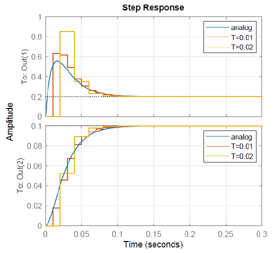
We observe from the figure that the armature current has a higher overshoot at the lower sampling rate, though both models display similar settling time of about 100 msec.

Pole Placement Design of Digital Controller

Given a discrete state variable model \(\left\{A_{\rm d},\ B_{\rm d}\right\}\), and a desired pulse characteristic polynomial \(\Delta _{\rm des} (z)\), a state feedback controller for the system can be designed using pole placement similar to that of the continuous-time system (Sec. 9.1.1).

Let the discrete-time model of a SISO system be given as:

\[{\bf x}_{k+1} ={\bf A}_{\rm d} {\bf x}_{k} +{\bf b}_{\rm d} u_{k} , \;\; y_{k} ={\bf c}^T {\bf x}_{k} \nonumber \]

A state feedback controller for the discrete state variable model is defined as:

\[u_k=-{\bf k}^T{\bf x}_k+r_k \nonumber \]

where \({\bf k}^{T}\) represents a row vector of constant feedback gains and \(r_k\) is a reference input sequence. The controller gains can be obtained by equating the coefficients of the characteristic polynomial with those of a desired polynomial:

\[\Delta (z)=\left|z{\bf I-A}_{\rm d} \right|=\Delta _{\rm des} (z) \nonumber \]

The \(\Delta _{\rm des} (z)\) above is a Hurwitz polynomial (in \(z\)), with roots inside the unit circle that meet given performance (damping ratio and/or settling time) requirements. Assuming that desired \(s\)-plane root locations are known, the corresponding \(z\)-plane root locations can be obtained from the equivalence: \(z=e^{Ts}\).

Closed-loop System

The closed-loop system model is given as:

\[{\bf x}_{k+1} ={\bf A}_{\rm cl} {\bf x}_{k} +{\bf b}_{\rm d} r_{k} , \;\; y_{k} ={\bf c}^T {\bf x}_{k} \nonumber \]

where \({\bf A}_{\rm cl} =({\bf A}_{\rm d}-{\bf b}_{\rm d}{\bf k}^T)\).

Assuming closed-loop stability, for a constant input \(r_k=r_{\rm ss}\), the steady-state response, \({\bf x}_{\rm ss}\), of the system obeys: 

\[{\bf x}_{ss} ={\bf A}_{\rm cl} {\bf x}_{ss} +{\bf b}_{\rm d} r_{ss} ,\;\; y_{\rm ss} ={\bf c}^T {\bf x}_{ss} \nonumber \]

Hence, \(y_{\rm ss}={\bf c}^T\,({\bf A}_{\rm cl}-{\bf I})^{-1}\,{\bf b}_{\rm d}\,r_{\rm ss}\).

Example \(\PageIndex{2}\)

The discrete state variable model of a DC motor (\(T=0.02\)s) is given as: \[\left[\begin{array}{c} {i_{k+1} } \\ {\omega _{k+1} } \end{array}\right]=\left[\begin{array}{cc} {0.134} & {-0.038} \\ {0.038} & {0.816} \end{array}\right]\left[\begin{array}{c} {i_{k} } \\ {\omega _{k} } \end{array}\right]+\left[\begin{array}{c} {0.863} \\ {0.053} \end{array}\right]V_{k} , \;\; y_{k} =\left[\begin{array}{cc} {0} & {1} \end{array}\right]\left[\begin{array}{c} {i_{k} } \\ {\omega _{k} } \end{array}\right] \nonumber \]

The desired \(s\)-plane root locations for the model are given as: \(s=-50,\; -100.\)

The corresponding \(z\)-plane roots (\(T=0.02s\)) are obtained as: \(z=e^{-1} ,\; e^{-2}\).

The desired characteristic polynomial is given as: \(\Delta _{\rm des} (z)=z^{2} -0.95z+0.05.\)

The feedback gains \(k^T =[k_{1} ,\; k_{2} ]\), computed using the MATLAB ‘place’ command, are given as: \(k_{1} =0.247,\; k_{2} =4.435.\)

The closed-loop system matrix is given as: \(A_\rm d)= \left[\begin{array}{cc} {-0.080} & {-3.867} \\ {0.025} & {0.583} \end{array}\right]\).

An update rule for implementation of the controller on computer is obtained as: \(u_{k} =-0.247\, i_{k} -4.435\, \omega _{k} .\)

The closed-loop response has steady-state value of \(\omega _{\rm ss}=0.143 \;\rm rad/s\).

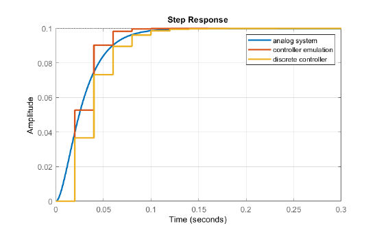
The step response of the closed-loop system is plotted in Figure 10.2.2, where the discrete system response was scaled to match the analog system response. The step response of the continuous-time system and that for the emulated controller gains are plotted alongside.

Figure \(\PageIndex{2}\): Unit-step response of the DC motor model for the following choices: analog system; controller emulation; digital controller.

Deadbeat Controller Design

A discrete-time system is called deadbeat if all closed-loop poles are placed at the origin \((z=0)\).

A deadbeat system has the remarkable property that its response reaches steady-state in \(n\)-steps, where \(n\) represents the model dimension.

The desired closed-loop pulse characteristic polynomial is selected as \(\Delta _{\rm des} (z)=z^{n}\).

To design a deadbeat controller, let the closed-loop pulse transfer function be defined as: \[T(z)=\frac{K(z)G(z)}{1+K(z)G(z)} \nonumber \]

The above equation is solved for \(K(z)\) to obtain: \[K(z)=\frac{1}{G(z)} \frac{T(z)}{1-T(z)} \nonumber \]

Let the desired \(T(z)=z^{-n}\); then, the deadbeat controller is given as: \[K(z)=\frac{1}{G(z)(z^{n} -1)} \nonumber \]

Example \(\PageIndex{3}\)

Let \(G(s)=\frac{1}{s+1} ;\) then \(G(z)=\frac{1-e^{-T} }{z-e^{-T} }\).

A deadbeat controller for the model is obtained as: \(K(z)=\frac{z-e^{-T} }{(1-e^{-T} )(z-1)}\).

Example \(\PageIndex{4}\)

The discrete state variable model of a DC motor for \(T=0.02\; \rm s\) is given as: \[\left[\begin{array}{c} {i_{k+1} } \\ {\omega _{k+1} } \end{array}\right]=\left[\begin{array}{cc} {0.134} & {-0.038} \\ {0.038} & {0.816} \end{array}\right]\left[\begin{array}{c} {i_{k} } \\ {\omega _{k} } \end{array}\right]+\left[\begin{array}{c} {0.863} \\ {0.053} \end{array}\right]V_{k} , \;\;y_{k} =\left[\begin{array}{cc} {0} & {1} \end{array}\right]\left[\begin{array}{c} {i_{k} } \\ {\omega _{k} } \end{array}\right] \nonumber \]

The state feedback controller is given as: \(u_{k} =-\left[k_{1} ,\, \, k_{2} \right]x_{k}\).

The closed-loop characteristic polynomial is obtained as: \[\Delta (z)=z^{2} +(0.863k_{1} +0.053k_{2} -0.95)z-0.707k_{1} +0.026k_{2} +0.111 \nonumber \]

For pole placement design, let \(\Delta _{\rm des} (z)=z^{2}\). By equating the polynomial coefficients, the deadbeat controller gains are obtained as: \(k_{1} =0.501,\; k_{2} =9.702\).

The update rule for controller implementation is given as: \[u_{k} =0.501\, \, i_{k} +9.702\, \, \omega _{k} \nonumber \]

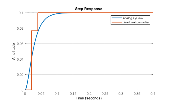
The step response of the deadbeat controller (Figure 10.2.3) settles in two time periods. The response was scaled to match that of the continuous-time system.

An approximate deadbeat design can be performed by choosing distinct closed-loop eigenvalues close to the origin, e.g., \(z=\pm {10}^{-5}\), and using the 'place' command from the MATLAB Control Systems Toolbox.

The feedback gains for the approximate design are obtained as: \(k_{1} =0.509,\; k_{2} =9.702\). The resulting closed-loop system response is still deadbeat.

Figure \(\PageIndex{3}\): The step response of the DC motor model with deadbeat controller. 

Feedforward Tracking System Design

A tracking system was previously designed by using feedforward cancelation of the error signal (Section 9.2.1). A similar design can be performed in the case of discrete systems.

Towards this end, let the discrete state variable model be given as: \[{\bf x}_{k+1} ={\bf A}_{\rm d} {\bf x}_{k} +{\bf b}_{\rm d} u_{k} , \;\;y_{k} ={\bf c}^T {\bf x}_{k} \nonumber \]

A tracking controller for the model is defined as: \[u_k=-{\bf k}^T{\bf x}_k+k_rr_k \nonumber \] where \({\bf k}^{T}\) represents a row vector of feedback gains, \(k_r\) is a feedforward gain, and \(r_k\) is a reference input sequence.

Assuming that a pole placement controller for the discrete system has been designed, the closed-loop system is given as: \[{\bf x}_{k+1}=\left({\bf A}_{\rm d}-{\bf b}_{\rm d}{\bf k}^T\right){\bf x}_k+{\bf b}_{\rm d}k_rr_k \nonumber \]

The closed-loop pulse transfer function is obtained as: \[T\left(z\right)={\bf c}^T_{\rm d}{\left(z{\bf I-A}_{\rm d}+{\bf b}_{\rm d}{\bf k}^T\right)}^{-1}{\bf b}_{\rm d}k_r \nonumber \] where \({\bf I}\) denotes an identity matrix. The condition for asymptotic tracking is given as: \[T\left(1\right)={\bf c}^T_{\rm d}{\left({\bf I-A}_{\rm d}+{\bf b}_{\rm d}{\bf k}^T\right)}^{-1}{\bf b}_{\rm d}k_r=1 \nonumber \]

The feedforward gain for error cancelation is obtained as: \(k_r=\frac{1}{T\left(1\right)}\).

Example \(\PageIndex{5}\)

The discrete state variable model of a DC motor (\(T=0.02\)s) is given as: \[\left[\begin{array}{c} {i_{k+1} } \\ {\omega _{k+1} } \end{array}\right]=\left[\begin{array}{cc} {0.134} & {-0.038} \\ {0.038} & {0.816} \end{array}\right]\left[\begin{array}{c} {i_{k} } \\ {\omega _{k} } \end{array}\right]+\left[\begin{array}{c} {0.863} \\ {0.053} \end{array}\right]V_{k} , \;\;y_{k} =\left[\begin{array}{cc} {0} & {1} \end{array}\right]\left[\begin{array}{c} {i_{k} } \\ {\omega _{k} } \end{array}\right] \nonumber \]

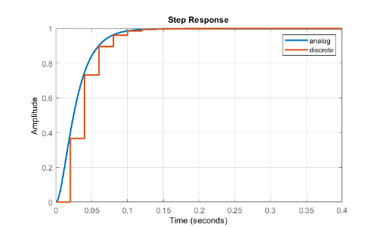
A state feedback controller for the motor model was previously designed as: \(k^T =[k_{1} ,\; k_{2} ]\), where \(k_{1} =0.247,\; k_{2} =4.435.\)

The closed-loop system is defined as: \[T\left(z\right)=\frac{0.367z+0.179}{z^2-0.503z+0.05}k_r \nonumber \]

From the asymptotic condition, the feedforward gain is solved as: \(k_r=6.98\).

The step response of the closed-loop system is shown in Figure 10.2.4.

Figure \(\PageIndex{4}\): The step response of the tracking controllers for the DC motor model.

Example \(\PageIndex{6}\)

The discrete state variable model of a DC motor (\(T=0.02\)s) is given as:

\[\left[\begin{array}{c} {i_{k+1} } \\ {\omega _{k+1} } \end{array}\right]=\left[\begin{array}{cc} {0.134} & {-0.038} \\ {0.038} & {0.816} \end{array}\right]\left[\begin{array}{c} {i_{k} } \\ {\omega _{k} } \end{array}\right]+\left[\begin{array}{c} {0.863} \\ {0.053} \end{array}\right]V_{k} , \;\;y_{k} =\left[\begin{array}{cc} {0} & {1} \end{array}\right]\left[\begin{array}{c} {i_{k} } \\ {\omega _{k} } \end{array}\right] \nonumber \]

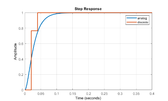
A dead-beat controller for the motor model was designed as: \(k^T =[k_{1} ,\; k_{2} ]\), where \(k_{1} =0.501,\; k_{2} =9.702\).

The closed-loop system is defined as: \[T\left(z\right)=\frac{0.672z+0.328}{z^2}k_r \nonumber \]

From the asymptotic condition, the feedforward gain is solved as: \(k_r=12.77\).

The step response of the closed-loop system is shown in Figure 10.2.5.

Figure \(\PageIndex{5}\): The step response of the deadbeat tracking controller for the DC motor model.

Tracking PI Controller Design

A tracking PI controller for the discrete state variable model is designed similar to the design of continuous-time system (Figure 9.3.1). The tracking PI controller places an integrator in the feedback loop, thus ensuring that the tracking error goes to zero in the steady-state.

In the case of continuous-time system, the tracking PI controller was defined as: \(u=-{\bf k}^{T} {\bf x}+k_{i} \int (r-y)\rm dt\).

Using the forward difference approximation to the integrator, given as: \(v_k=v_{k-1}+Te_k\), an augmented discrete-time system model including the integrator state variable is formed as:

\[\left[\begin{array}{c} {{\bf x}(k+1)} \\ {v(k+1)} \end{array}\right]=\left[\begin{array}{cc} {{\bf A}_{\rm d} } & {\bf 0} \\ {-{\bf c}^T T} & {1} \end{array}\right] \left[\begin{array}{c} {{\bf x}(k)} \\ {v(k)} \end{array}\right]+\left[\begin{array}{c} {{\bf b}_{\rm d} } \\ {0} \end{array}\right]u+\left[\begin{array}{c} {\bf 0} \\ {T} \end{array}\right]r \nonumber \]

The state feedback controller for the augmented system is defined as:

\[u(k)=\left[\begin{array}{cc} {-{\bf k}^T } & {k_ i } \end{array}\right]\, \left[\begin{array}{c} {{\bf x}(k)} \\ {v(k)} \end{array}\right] \nonumber \]

where \(k_ i\) represents the integral gain. With the addition of the above controller, the closed-loop system is described as:

\[\left[\begin{array}{c} {{\bf x}(k+1)} \\ {v(k+1)} \end{array}\right]=\left[\begin{array}{cc} {{\bf A}_{\rm d} -{\bf b}_{\rm d} k^{T} } & {{\bf b}_{\rm d} k_{i} } \\ {-{\bf c}^T T} & {1} \end{array}\right] \left[\begin{array}{c} {{\bf x}(k)} \\ {v(k)} \end{array}\right]+\left[\begin{array}{c} {\bf 0} \\ {T} \end{array}\right]r(k) \nonumber \]

The closed-loop characteristic polynomial of the augmented system is formed as:

\[{\mathit{\Delta}}_a\left(z\right)=\left| \begin{array}{cc} z{\bf I-A}_{\rm d}+{\bf b}_{\rm d}k^T & -{\bf b}_{\rm d}k_i \\ -{\bf c}^T_{\rm d}T & z-1 \end{array} \right| \nonumber \]

where \({\bf I}\) denotes an identity matrix of order \(n\).

Next, we choose a desired characteristic polynomial of \((n+1)\) order, and perform pole placement design for the augmented system. The location of the integrator pole in the \(z\)-plane may be selected keeping in view the desired peformance criteria for the closed-loop system.

Example \(\PageIndex{6}\)

The discrete state variable model of a DC motor (\(T=0.02\)s) is given as:

\[\left[ \begin{array}{c} i_{k+1} \\ {\omega }_{k+1} \end{array} \right]=\left[ \begin{array}{cc} 0.134 & -0.038 \\ 0.038 & 0.816 \end{array} \right]\left[ \begin{array}{c} i_k \\ {\omega }_k \end{array} \right]+\left[ \begin{array}{c} 0.863 \\ 0.053 \end{array} \right]V_k,\ \ {\omega }_k=\left[ \begin{array}{cc} 0 & 1 \end{array} \right]\left[ \begin{array}{c} i_k \\ {\omega }_k \end{array} \right] \nonumber \]

The control law for the tracking PI controller is defined as:

\[u_k=-k_1i_k-k_2{\omega }_k+k_iv_k \nonumber \]

where \(v_{k} =v_{k-1} +T(r_{k} -\omega _{k} )\) describes the output of the integrator. The augmented system model for the pole placement design using integral control is given as:

\[\left[ \begin{array}{c} i_{k+1} \\ {\omega }_{k+1} \\ v_{k+1} \end{array} \right]=\left[ \begin{array}{ccc} 0.134 & -0.038 & 0 \\ 0.038 & 0.816 & 0 \\ 0 & -0.02 & 1 \end{array} \right]\left[ \begin{array}{c} i_k \\ {\omega }_k \\ v_k \end{array} \right]+\left[ \begin{array}{c} 0.863 \\ 0.053 \\ 0 \end{array} \right]V_k+\left[ \begin{array}{c} 0 \\ 0 \\ 0.02 \end{array} \right]r_k \nonumber \]

The desired \(z\)-plane pole locations for a desired \(\zeta=0.7\) are selected as: \(z=e^{-1} ,\; e^{-1\pm j1}\).

The controller gains, obtained using the MATLAB ‘place’ command, are given as: \(k_{1} =0.43,k_{2} =15.44,\; k_{i} =-297.79.\)

An update rule for controller implementation on computer is given as:

\[u_k=-0.43i_k-15.44{\omega }_k+297.8v_k \nonumber \]

\[v_k=v_{k-1}+0.02\left(r_k-{\omega }_k\right) \nonumber \]

The step response of the closed-loop system is plotted in Figure 10.2.6. The step response of the continuous-time system (Example 9.1.1) is plotted alongside. The output in both cases attains steady-state value of unity in about 0.12sec.

Figure \(\PageIndex{6}\): Tracking PI control of the DC motor model: closed-loop response for the analog and discrete systems.