
5.1: Four Questions
- Page ID
- 81494

\( \newcommand{\vecs}[1]{\overset { \scriptstyle \rightharpoonup} {\mathbf{#1}} } \)
\( \newcommand{\vecd}[1]{\overset{-\!-\!\rightharpoonup}{\vphantom{a}\smash {#1}}} \)
\( \newcommand{\dsum}{\displaystyle\sum\limits} \)
\( \newcommand{\dint}{\displaystyle\int\limits} \)
\( \newcommand{\dlim}{\displaystyle\lim\limits} \)
\( \newcommand{\id}{\mathrm{id}}\) \( \newcommand{\Span}{\mathrm{span}}\)
( \newcommand{\kernel}{\mathrm{null}\,}\) \( \newcommand{\range}{\mathrm{range}\,}\)
\( \newcommand{\RealPart}{\mathrm{Re}}\) \( \newcommand{\ImaginaryPart}{\mathrm{Im}}\)
\( \newcommand{\Argument}{\mathrm{Arg}}\) \( \newcommand{\norm}[1]{\| #1 \|}\)
\( \newcommand{\inner}[2]{\langle #1, #2 \rangle}\)
\( \newcommand{\Span}{\mathrm{span}}\)
\( \newcommand{\id}{\mathrm{id}}\)
\( \newcommand{\Span}{\mathrm{span}}\)
\( \newcommand{\kernel}{\mathrm{null}\,}\)
\( \newcommand{\range}{\mathrm{range}\,}\)
\( \newcommand{\RealPart}{\mathrm{Re}}\)
\( \newcommand{\ImaginaryPart}{\mathrm{Im}}\)
\( \newcommand{\Argument}{\mathrm{Arg}}\)
\( \newcommand{\norm}[1]{\| #1 \|}\)
\( \newcommand{\inner}[2]{\langle #1, #2 \rangle}\)
\( \newcommand{\Span}{\mathrm{span}}\) \( \newcommand{\AA}{\unicode[.8,0]{x212B}}\)
\( \newcommand{\vectorA}[1]{\vec{#1}} % arrow\)
\( \newcommand{\vectorAt}[1]{\vec{\text{#1}}} % arrow\)
\( \newcommand{\vectorB}[1]{\overset { \scriptstyle \rightharpoonup} {\mathbf{#1}} } \)
\( \newcommand{\vectorC}[1]{\textbf{#1}} \)
\( \newcommand{\vectorD}[1]{\overrightarrow{#1}} \)
\( \newcommand{\vectorDt}[1]{\overrightarrow{\text{#1}}} \)
\( \newcommand{\vectE}[1]{\overset{-\!-\!\rightharpoonup}{\vphantom{a}\smash{\mathbf {#1}}}} \)
\( \newcommand{\vecs}[1]{\overset { \scriptstyle \rightharpoonup} {\mathbf{#1}} } \)
\(\newcommand{\longvect}{\overrightarrow}\)
\( \newcommand{\vecd}[1]{\overset{-\!-\!\rightharpoonup}{\vphantom{a}\smash {#1}}} \)
\(\newcommand{\avec}{\mathbf a}\) \(\newcommand{\bvec}{\mathbf b}\) \(\newcommand{\cvec}{\mathbf c}\) \(\newcommand{\dvec}{\mathbf d}\) \(\newcommand{\dtil}{\widetilde{\mathbf d}}\) \(\newcommand{\evec}{\mathbf e}\) \(\newcommand{\fvec}{\mathbf f}\) \(\newcommand{\nvec}{\mathbf n}\) \(\newcommand{\pvec}{\mathbf p}\) \(\newcommand{\qvec}{\mathbf q}\) \(\newcommand{\svec}{\mathbf s}\) \(\newcommand{\tvec}{\mathbf t}\) \(\newcommand{\uvec}{\mathbf u}\) \(\newcommand{\vvec}{\mathbf v}\) \(\newcommand{\wvec}{\mathbf w}\) \(\newcommand{\xvec}{\mathbf x}\) \(\newcommand{\yvec}{\mathbf y}\) \(\newcommand{\zvec}{\mathbf z}\) \(\newcommand{\rvec}{\mathbf r}\) \(\newcommand{\mvec}{\mathbf m}\) \(\newcommand{\zerovec}{\mathbf 0}\) \(\newcommand{\onevec}{\mathbf 1}\) \(\newcommand{\real}{\mathbb R}\) \(\newcommand{\twovec}[2]{\left[\begin{array}{r}#1 \\ #2 \end{array}\right]}\) \(\newcommand{\ctwovec}[2]{\left[\begin{array}{c}#1 \\ #2 \end{array}\right]}\) \(\newcommand{\threevec}[3]{\left[\begin{array}{r}#1 \\ #2 \\ #3 \end{array}\right]}\) \(\newcommand{\cthreevec}[3]{\left[\begin{array}{c}#1 \\ #2 \\ #3 \end{array}\right]}\) \(\newcommand{\fourvec}[4]{\left[\begin{array}{r}#1 \\ #2 \\ #3 \\ #4 \end{array}\right]}\) \(\newcommand{\cfourvec}[4]{\left[\begin{array}{c}#1 \\ #2 \\ #3 \\ #4 \end{array}\right]}\) \(\newcommand{\fivevec}[5]{\left[\begin{array}{r}#1 \\ #2 \\ #3 \\ #4 \\ #5 \\ \end{array}\right]}\) \(\newcommand{\cfivevec}[5]{\left[\begin{array}{c}#1 \\ #2 \\ #3 \\ #4 \\ #5 \\ \end{array}\right]}\) \(\newcommand{\mattwo}[4]{\left[\begin{array}{rr}#1 \amp #2 \\ #3 \amp #4 \\ \end{array}\right]}\) \(\newcommand{\laspan}[1]{\text{Span}\{#1\}}\) \(\newcommand{\bcal}{\cal B}\) \(\newcommand{\ccal}{\cal C}\) \(\newcommand{\scal}{\cal S}\) \(\newcommand{\wcal}{\cal W}\) \(\newcommand{\ecal}{\cal E}\) \(\newcommand{\coords}[2]{\left\{#1\right\}_{#2}}\) \(\newcommand{\gray}[1]{\color{gray}{#1}}\) \(\newcommand{\lgray}[1]{\color{lightgray}{#1}}\) \(\newcommand{\rank}{\operatorname{rank}}\) \(\newcommand{\row}{\text{Row}}\) \(\newcommand{\col}{\text{Col}}\) \(\renewcommand{\row}{\text{Row}}\) \(\newcommand{\nul}{\text{Nul}}\) \(\newcommand{\var}{\text{Var}}\) \(\newcommand{\corr}{\text{corr}}\) \(\newcommand{\len}[1]{\left|#1\right|}\) \(\newcommand{\bbar}{\overline{\bvec}}\) \(\newcommand{\bhat}{\widehat{\bvec}}\) \(\newcommand{\bperp}{\bvec^\perp}\) \(\newcommand{\xhat}{\widehat{\xvec}}\) \(\newcommand{\vhat}{\widehat{\vvec}}\) \(\newcommand{\uhat}{\widehat{\uvec}}\) \(\newcommand{\what}{\widehat{\wvec}}\) \(\newcommand{\Sighat}{\widehat{\Sigma}}\) \(\newcommand{\lt}{<}\) \(\newcommand{\gt}{>}\) \(\newcommand{\amp}{&}\) \(\definecolor{fillinmathshade}{gray}{0.9}\)Newton's second law, commonly written as \(F=m a\), is one of the most famous relations in physics. This relation, along with Newton's first and third laws, is typically the starting point for mechanics instruction in high school and undergraduate physics. Mechanics instruction is often broken down into three different areas: forces in stationary systems, motion of a particle subjected to a force, and impact problems. By focusing on each area individually, it is possible to begin to develop a physical understanding of the important physical phenomena.
When engineers apply these principles to realistic problems, they find it helpful to have a more general framework, one that provides a common basis for developing useful mathematical models. To provide this framework, we develop a physical law called the Conservation of Linear Momentum that, with few restrictions, is universally applicable. Then, as we did with mass and charge, we will explore the modeling assumptions that engineers commonly use when they build mathematical models of physical systems.
When developing an accounting concept for a new property, there are four questions that must be answered. When applied to linear momentum, the questions become
- What is linear momentum?
- How can linear momentum be stored in a system?
- How can linear momentum be transported?
- How can linear momentum be created or destroyed?
Once we have answered these questions we will have the appropriate accounting equation for the linear momentum of a system.
What is linear momentum?
As a starting point, let's consider the motion of a very specialized system, a particle. A particle is a closed system that behaves as if its volume was negligible and its mass was concentrated at a single point. The motion of a particle is completely described by its velocity, and all interactions between a particle and its surroundings occur at a single point. Later we will consider more realistic and larger extended systems for which the particle assumption is insufficient; however, we will find that the particle assumption is often a very good model.
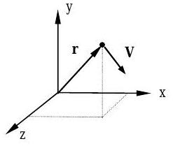
Figure \(\PageIndex{1}\): Particle with mass \(m\) at position \(\mathbf{r}\) with velocity \(\mathbf{V}\).
For a particle with mass \(m\) and velocity \(\mathbf{V}\) as shown Figure \(\PageIndex{1}\), the linear momentum of the particle, \(\mathrm{P}\), is defined as the product of the particle mass and the particle velocity: \[\mathbf{P}=m \mathbf{V} \nonumber \] The dimensions of linear momentum in terms of primary dimensions are the product of the dimensions of mass and velocity, \([\mathrm{M}][\mathrm{L}] /[\mathrm{T}]\). Typical units for linear momentum are \(\mathrm{kg} \cdot \mathrm{m} / \mathrm{s}\) in SI and \(\mathrm{slug} \cdot \mathrm{ft} / \mathrm{s}\) (or \(\mathrm{lbm} \cdot \mathrm{ft} / \mathrm{s}\)) in USCS.
It is important to note that the linear momentum \(\mathbf{P}\), like velocity \(\mathbf{V}\), is a vector. As shown in Figure \(\PageIndex{2}\), vectors are typically represented by arrows. A vector is a mathematical expression that has a magnitude, a direction, and adds according to the parallelogram law. The magnitude of the vector describes the "length" of the arrow, and if it represents a physical quantity, the magnitude includes both a number and the associated units. The direction of a vector is specified in terms of its line of action and its sense. As shown in Figure \(\PageIndex{2}\) vectors \(\mathbf{P}_{\mathrm{A}}\) and \(\mathbf{P}_{\mathrm{B}}\) have the same magnitude and same line of action but opposite sense. The magnitude of a vector is a positive number and is represented mathematically as \(P_{A}=\left| \mathbf{P}_{A} \right|\). The complete vector is described by giving the magnitude and the direction of each vector: \(\mathbf{P}_{A} = P_{A} \ \angle \theta=(5 \mathrm{~kg} \cdot \mathrm{m} / \mathrm{s}) \ \angle \theta\) and \(\mathbf{P}_{B}=P_{B} \ \angle (\theta+\pi)=(5 \mathrm{~kg} \cdot \mathrm{m} / \mathrm{s}) \ \angle(\theta+\pi)\), where all angles are measured from the reference line.
.jpg?revision=1)
Figure \(\PageIndex{2}\): Magnitude and direction of a vector.
In addition to magnitude and direction, vectors that represent linear momentum and its transport also have a point of application. A vector with a point of application is called a bound vector. In summary, a linear momentum vector is completely specified on]ce we know its magnitude, direction, and point of application.
Because the linear momentum of a particle depends upon its mass, linear momentum is an extensive property. As with other extensive properties linear momentum has an intensive form. The linear momentum per unit mass, or the specific linear momentum \(\mathbf{p}\), is defined as \[\mathbf{p} \equiv \lim _{V\kern-0.5em\raise0.3ex-_{\mathrm{sys}} \rightarrow 0} \frac{\mathbf{P}_{\mathrm{sys}}}{m_{\mathrm{sys}}}=\mathbf{V} \nonumber \] Thus the velocity of a particle is really just the specific linear momentum of particle.
It is important to note that velocity, like position, is always measured relative to a reference point. When used to define the linear momentum, the velocity must be measured relative to an inertial reference frame. For our purposes this means a coordinate system that is not rotating or accelerating with respect to the Earth, i.e. an Earth-fixed coordinate system. In addition, any coordinate system that is moving with a constant velocity with respect to the Earth is also an inertial reference frame.
As we will show later, it is frequently useful to attach the coordinate system to a moving system if the system is moving with a constant velocity. Under these conditions all velocities are computed relative to the moving coordinate system. For motion of spacecraft you would need to use a Sun-centered, non-rotating reference frame. See any undergraduate physics textbook to learn more about the conditions of an inertial reference frame.
5.1.1 Kinematics of a particle
Because of the relationship of velocity to linear momentum, an understanding of kinematics will play a crucial role in our study of linear momentum. Kinematics is the study of the geometry of motion without regard to the cause of the motion and provides the relationship between the position \(\mathrm{r}\), velocity \(\mathrm{V}\), and acceleration \(\mathrm{a}\) of a point. The velocity vector \(\mathrm{V}\) is related to the position vector \(\mathrm{r}\) through the basic kinematic relationship you learned in physics—velocity is the first derivative of position:
\[\mathbf{V}=\frac{d \mathbf{r}}{d t} \nonumber \] The dimensions of velocity are length per unit time, \([\mathrm{L}] / [\mathrm{T}]\). Typical units for velocity are \(\mathrm{m} / \mathrm{s}\) in SI or \(\mathrm{ft} / \mathrm{s}\) in USCS.
The first derivative of velocity (or the second derivative of position) is the acceleration vector \(\mathbf{a}\) : \[\mathbf{a}=\frac{d \mathbf{V}}{dt} = \frac{d}{dt} \left( \frac{d \mathbf{r}}{dt} \right) \nonumber \] The dimensions of acceleration are length per unit time squared, \([\mathrm{L}] /[\mathrm{T}]^{2}\). Typical units for acceleration are \(\mathrm{m} / \mathrm{s}^{2}\) in SI or \(\mathrm{ft} / \mathrm{s}^{2}\) in USCS.
Rectilinear motion
In rectilinear motion, a particle can only move along a straight line. Under these conditions only one spatial coordinate, say \(x\), is required to describe the particle position, and the velocity and acceleration are written as \[V=\frac{dx}{dt} \quad \text { and } \quad a=\frac{dV}{dt}=\frac{d^{2} x}{d t^{2}} \nonumber \] These relationships are most useful when position \(x\), velocity \(V\), and acceleration \(a\) are all functions of time. Under conditions of rectilinear motion, a positive numerical value for the velocity implies that the particle is moving in the same direction as the positive \(x\)-axis. Similarly, a positive numerical value for the acceleration implies that the velocity of the particle is increasing as it moves in the direction of the positive \(x\)-axis.
An alternate expression for acceleration is sometimes useful if acceleration and velocity are known as functions of position, e.g. \(V=V(x)\) and \(a=a(x)\). Under these conditions the acceleration can be written as \[\begin{array} x &= f_{x}(t) \\ V &= f_{V}(x) \quad \rightarrow \quad a \equiv \frac{dV}{dt}=\overbrace{ \left( \frac{dV}{dx} \right) \underbrace{ \left( \frac{dx}{dt} \right)}_{=V} }^{\text {Chain Rule of Differentiation}} =V \frac{d V}{d x} \\ a &= f_{a}(x) \end{array} \nonumber \] using the chain rule of differentiation from calculus. Note that the notation "\(f(t)\)" is read as "a function of \(t\)."
One of the common tasks of kinematics is to integrate the acceleration (time rate of change, or first derivative, of velocity) of a point with respect to time or with respect to position. Do not memorize the formulas described below. Each of the results is different but the approach is the same. Learn the process, not the result!
Case I: Acceleration is known as a function of time, e.g. \(a=f(t)\). To find the velocity, integrate with respect to time as follows: \[a = f(t) = \frac{dV}{dt} \rightarrow dV = f(t) dt \quad \rightarrow \quad V - V_{o} = \int\limits_{t_o}^t f(t) \ dt \nonumber \]
Practice: (a) Given that \(a=bt\) and \(V=V_{o}\) at \(t=0 \mathrm{~s}\), develop an equation for the velocity \(V\). (b) Determine the velocity at \(t=5 \mathrm{~s}\), if \(b=15 \mathrm{~m} / \mathrm{s}^{3}\) and \(V_{o}=20 \mathrm{~m} / \mathrm{s}\).
Case II: Acceleration is known as a function of position, e.g. \(a=f(x)\). The velocity can be determined by integrating with respect to position as below: \[a = f(x) = V \frac{dV}{dx} \quad \rightarrow \quad V \ dV = f(x) dx \quad \rightarrow \quad \frac{V^2}{2}-\frac{V_{o}^2}{2} = \int\limits_{x_{o}}^{x} f(x) \ dx \nonumber \]
Practice: (a) Given that \(a=c x\) and \(V=V_{o}\) at \(x=0\), develop an equation for the velocity \(V\). (b) Determine the velocity at \(x=5 \mathrm{~m}\), if \(c=10 \mathrm{~s}^{-2}\) and \(V_{o}=10 \mathrm{~m} / \mathrm{s}\).
Case III: Acceleration is known as a function of velocity, e.g. \(a=f(V)\). The velocity can be determined by integrating with respect to time or position as below: \[\begin{align*} & a = f(V) = \frac{dV}{dt} &\rightarrow \quad & dt = \frac{dV}{f(V)} &\rightarrow \quad & t - t_{o} = \int\limits_{V_o}^{V} \frac{dV}{f(V)} \\ & a = f(V) = V \frac{dV}{dx} &\rightarrow \quad & dx =\left[ \frac{V}{f(V)} \right] dV &\rightarrow \quad & x - x_{o} = \int_{V_o}^{V} \left[ \frac{V}{f(V)} \right] \ dV \end{align*} \nonumber \]
Practice: (a) Given that \(a=b V^2\) and \(V=V_{o}\) at \(x=x_{o}\), develop an equation for the velocity \(V\). (b) Given that \(a=b V^2\) and \(V=V_{0}\) at \(t=t_{o}\), develop an equation for the velocity \(V\).
Case IV: Acceleration is a constant, e.g. \(a = \text{constant}\). The velocity can be determined by integrating with respect to time or position as below: \[ a=\text { constant } \quad \rightarrow \quad \begin{array} a a = \dfrac{d V}{d t} & \rightarrow & dV = a \ dt \quad\quad \rightarrow \quad V - V_{o} = a \left( t-t_{o} \right) \\ a=V \dfrac{dV}{dx} & \rightarrow & V \ dV = a \ dx \quad \rightarrow \quad \dfrac{V^2}{2}-\dfrac{V_{o}^2}{2} = a \left( x-x_{o} \right) \end{array} \nonumber \]
Practice: Starting with the definition of velocity \(V = d x / d t\), prove that the position can be described by an equation of the form \(x - x_{o} = V_{o} t +(1 / 2) a t^{2}\).
Plane curvilinear motion
In plane (or two-dimensional) curvilinear motion, the motion is constrained to a plane. Writing the position vector \(\mathbf{r}\) (Figure \(\PageIndex{3}\)) for a point in the plane in terms of its rectangular components gives \[\mathbf{r} = x \mathbf{i} + y \mathbf{j} \nonumber \] where \(\mathbf{i}\) and \(\mathbf{j}\) are the two orthogonal unit vectors and \(x\) and \(y\) are the corresponding distances measured in the direction of each unit vector.
.png?revision=1)
Figure \(\PageIndex{3}\): Rectangular coordinates
Differentiating Eq. \(\PageIndex{7}\) as required by Eq. \(\PageIndex{3}\) gives the velocity vector in terms of its components
\[\begin{align} \mathbf{V} &= \frac{d}{dt} (x \mathbf{i} + y \mathbf{j}) \nonumber \\[4pt] &=\frac{d(x \mathbf{i})}{dt} + \frac{d(y \mathbf{j})}{dt} = \left( \frac{dx}{dt} \mathbf{i} +x \cancel{ \frac{d \mathbf{i}}{dt} }^{=0} \right) + \left( \frac{dy}{dt} \mathbf{j} + y \cancel{ \frac{d \mathbf{j}}{dt} }^{=0} \right) \\[4pt] &= \left( \frac{dx}{dt} \right) \mathbf{i} + \left(\frac{dy}{dt}\right) \mathbf{j} \nonumber \\[4pt] &=V_{x} \mathbf{i} + V_{y} \mathbf{j} \nonumber \end{align} \nonumber \]
where \(V_{x}\) and \(V_{y}\) are the velocity components in the \(x\) and \(y\) directions, respectively. Recall from your study of calculus that the derivative of a constant, such as the unit vector \(\mathbf{i}\), is identically zero. Similarly, it can be shown that the acceleration vector has the components: \[\begin{align} \mathbf{a} &=\frac{d \mathbf{V}}{dt} = \frac{d}{dt} \left( V_{x} \mathbf{i} + V_{y} \mathbf{j} \right) \nonumber \\[4pt] &=\frac{d V_{x}}{dt} \mathbf{i} + \frac{d V_{y}}{dt} \mathbf{j} \\[4pt] &=a_{x} \mathbf{i} + a_{y} \mathbf{j} \nonumber \end{align} \nonumber \] where \(a_{x}\) and \(a_y\) are the velocity components in the \(x\) and \(y\) directions, respectively.
Relative Motion
Recall that when you are computing the linear momentum of a system all velocities must be measured with respect to an inertial, i.e. non-accelerating, reference frame. Thus, if the velocity is measured in an accelerating reference frame, it will be necessary to determine the absolute velocity before we can compute the system linear momentum. Furthermore, if a system is translating with constant velocity, it will sometimes simplify a problem to compute the linear momentum with respect to this moving, inertial reference frame.
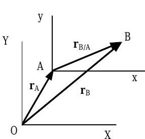
Figure \(\PageIndex{4}\): Relative position.
The relative position vector \(\mathbf{r}_{B / A}\) of point \(B\) with respect to point \(A\) (See Figure \(\PageIndex{4}\)) is defined by the relation: \[ \mathbf{r}_{B/A} = \mathbf{r}_B - \mathbf{r}_A \nonumber \]
where the position vector \(\mathbf{r}_A\) of point \(A\) and position vector \(\mathbf{r}_B\) of point \(B\) are both measured with respect to point \(O\), the origin of coordinate system XYZ. Given the relative position of point \(B\) with respect to point \(A\) and the absolute position of point \(A\), Eq. \(\PageIndex{10}\) can be rewritten as below to find the absolute velocity of point \(B\) : \[\mathbf{r}_{B} = \mathbf{r}_{A}+\mathbf{r}_{B / A} \nonumber \]
Similar relations can be written for the relative and absolute velocities of points \(A\) and \(B\) : \[\begin{align} \mathbf{V}_{B / A} = \mathbf{V}_{B} - \mathbf{V}_{A} & \rightarrow & \mathbf{V}_{B} = \mathbf{V}_{A} + \mathbf{V}_{B / A} \\ \mathbf{a}_{B / A} = \mathbf{a}_{B} - \mathbf{a}_{A} & \rightarrow & \mathbf{a}_{B} = \mathbf{a}_{A} + \mathbf{a}_{B / A} \end{align} \nonumber \]
Imagine that a railroad flatcar is accelerating and moving to the right with an instantaneous velocity of \(5 \mathrm{~m} / \mathrm{s}\) as measured by an observer on the ground. A forklift located on the bed of the flatcar is moving with a velocity of \(3 \mathrm{~m} / \mathrm{s}\) as measured by an observer sitting on the moving flatcar. Both observers see left and right directions similarly.
Determine the absolute velocity of the forklift, i.e. the velocity of the forklift as measured by an observer on the ground,
(a) if the observer sitting on the flatcar sees the forklift moving to her left and
(b) if the observer sitting on the flatcar sees the forklift moving to her right.
Solution
The following equation defines the relative velocity of the forklift with respect to the flatcar: \[\mathbf{V}_{\text {forklift / flat car}} = \mathbf{V}_{\text {forklift}} - \mathbf{V}_{\text {flatcar}} \quad \rightarrow \quad \mathbf{V}_{\text {forklift}} = \mathbf{V}_{\text {flatcar}} + \mathbf{V}_{\text {forklift / flatcar}} \nonumber \]
Now assume that the positive axis for our coordinate system points to the right.
(a)
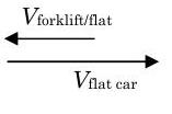
Figure \(\PageIndex{5}\): Forklift moves to the left as observed by an observer on the flat car.
\[\begin{aligned} \rightarrow + \quad V_{\text {forklift}} &= V_{\text {flatcar}} -V_{\text {forklift / flatcar}} \\ &=(5 \mathrm{~m} / \mathrm{s}) - (3 \mathrm{~m} / \mathrm{s}) \\ &= 2 \mathrm{~m} / \mathrm{s} \\ \mathbf{V}_{\text {forklift}} &= 2 \mathrm{~m} / \mathrm{s} \text { to the right.} \end{aligned} \nonumber \]
(b)
.png?revision=1)
Figure \(\PageIndex{6}\): Forklift moves to the right as observed by an observer on the flat car.
\[\begin{aligned} \rightarrow+ \quad V_{\text {forklift}} &= V_{\text {flatcar}} + V_{\text {forklift / flatcar}} \\ &= (5 \mathrm{~m} / \mathrm{s}) + (3 \mathrm{~m} / \mathrm{s}) \\ &= 8 \mathrm{~m} / \mathrm{s} \\ \mathbf{V}_{\text {forklift}} &= 8 \mathrm{~m} / \mathrm{s} \text { to the right.} \end{aligned} \nonumber \]
5.1.2 How can linear momentum be stored in a system?
Linear momentum is stored in the motion of the mass of a system; thus any system that has mass has the ability to store linear momentum. Because it is an extensive property, the linear momentum of a system can be found by adding up the linear momentum of each mass inside the system. For a system consisting of \(\mathrm{N}\) particles, the linear momentum of the system \(\mathbf{P}_{\text {sys}}\) is found by summing the linear momentum of the \(\mathbf{N}\) particles in the system, \[\mathbf{P}_{\mathrm{sys}} = \sum_{j=1}^{N} \mathbf{P}_{j} = \sum_{j=1}^{N} m_{j} \mathbf{V}_{j} \nonumber \]
For a continuous system, this summation is performed using an integral over the system volume: \[\mathbf{P}_{\mathrm{sys}}=\int\limits_{V\kern-0.5em\raise0.3ex-_{\mathrm{sys}}} ( \mathbf{V} \rho) \ d V\kern-0.8em\raise0.3ex- \nonumber \] where in general velocity and density can vary with both time and position.
Center of mass
To calculate the linear momentum for an extended system, i.e. something other than a particle, it is necessary to evaluate the integral in Eq. \(\PageIndex{15}\). Fortunately this process can be greatly simplified by introducing the concept of center of mass. The center of mass is the point where all of the mass for a system can be assumed to be concentrated for purposes of calculating the linear momentum. As we will show later, this makes the evaluation of the linear momentum a simpler task.
The velocity of the center of mass, \(\mathbf{V}_{G}\), is defined by the following equation: \[\mathbf{P}_{sys} = m_{sys} \mathbf{V}_{G} \equiv \int\limits_{V\kern-0.5em\raise0.3ex-_{sys}} (\mathbf{V} \rho) \ d V\kern-0.8em\raise0.3ex- \quad \rightarrow \quad \mathbf{V}_{G} = \frac{1}{m_{sys}} \int\limits_{V\kern-0.5em\raise0.3ex-_{sys}} (\mathbf{V} \rho) \ d V\kern-0.8em\raise0.3ex- \nonumber \] Thus the velocity of the center of mass equals the linear momentum of the system divided by the mass of the system.
The position of the center of mass, \(\mathbf{r}_{G}\), is the mass-weighted average of the position of all of the mass within the system: \[\mathbf{r}_{G} = \frac{1}{m_{sys}} \int\limits_{V\kern-0.5em\raise0.3ex-_{sys}} \mathbf{r} \rho \ d V\kern-0.8em\raise0.3ex- \nonumber \] On the surface of the earth, the location of the center of mass is essentially the same as the location of the center of gravity. From experience, we know that an object suspended from its center of gravity has no tendency to rotate, i.e. it is perfectly balanced. When the density of a system is uniform, the location of the center of mass is identical with the centroid of the volume of the system. The location of the centroid for most common shapes has been tabulated and can be found in mathematical and physical handbooks.
A system consists of three particles with mass, velocity, and positions as indicated in the table.
| Particle | \( m \ \text{(kg)}\) | \(\mathbf{r} \ \text{(m)}\) | \(\mathbf{V} \ \text{(m} / \text{s)}\) |
|---|---|---|---|
| 1 | \(15\) | \(3 \mathbf{i} + 3 \mathbf{j}\) | \(5 \mathbf{i} + 5 \mathbf{j}\) |
| 2 | \(10\) | \(-4 \mathbf{i} + 2 \mathbf{j}\) | \(3 \mathbf{i} - 5 \mathbf{j}\) |
| 3 | \(5\) | \(1 \mathbf{i} + 2 \mathbf{j}\) | \(2 \mathbf{i} - 2 \mathbf{j}\) |
Determine the following for the system:
(a) Linear momentum, in \(\mathrm{kg} \cdot \mathrm{m} / \mathrm{s}\).
(b) Velocity of the center of mass, in \(\mathrm{m} / \mathrm{s}\).
(c) Location of the center of mass, in \(\mathrm{m}\).
Solution
Known: Description of a system with pertinent information
Find: Calculate the linear momentum for each system.
Given: See below in each example.
Analysis
(a) Use the definition of linear momentum.
\[\begin{aligned} \mathbf{P}_{\mathrm{sys}} &= \mathbf{P}_{1} + \mathbf{P}_{2} + \mathbf{P}_{3} \\ &=m_1 \mathbf{V}_{1} +m_2 \mathbf{V}_{2} + m_3 \mathbf{V}_{3} \\ &= (15 \mathrm{~kg}) \left[ \left( 5 \ \frac{\mathrm{m}}{\mathrm{s}} \right) \mathbf{i} + \left( 5 \ \frac{\mathrm{m}}{\mathrm{s}} \right) \mathbf{j} \right] + (10 \mathrm{~kg}) \left[ \left( 3 \ \frac{\mathrm{m}}{\mathrm{s}} \right) \mathbf{i} - \left(5 \ \frac{\mathrm{m}}{\mathrm{s}} \right) \mathbf{j} \right] + (5 \mathrm{~kg}) \left[ \left( 2 \ \frac{\mathrm{m}}{\mathrm{s}} \right) \mathbf{i} - \left(2 \ \frac{\mathrm{m}}{\mathrm{s}} \right) \mathbf{j} \right] \\ &= \left[ (75+30+10) \mathbf{i} + (75-50-10) \mathbf{j} \right] \left(\frac{\mathrm{kg} \cdot \mathrm{m}}{\mathrm{s}} \right) \\ &= (115 \mathbf{i} + 15 \mathbf{j}) \left( \frac{\mathrm{kg} \cdot \mathrm{m}}{\mathrm{s}}\right) \text { or } \left( 115 \ \frac{\mathrm{kg} \cdot \mathrm{m}}{\mathrm{s}} \right) \mathbf{i} + \left( 15 \ \frac{\mathrm{kg} \cdot \mathrm{m}}{\mathrm{s}} \right) \mathbf{j} \end{aligned} \nonumber \]
(b) Use the defining equation for velocity of the center of mass
(c) Use the defining equation for location of center of mass
Plane motion of a rigid body
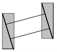
Many physical systems of interest can be modeled as a rigid body. A rigid body is a body that does not deform, i.e., the relative distance between any two points on the body remains a constant.
In this course we will restrict most of our discussions to what is referred to as plane motion. Plane motion occurs when any point in the body travels in a plane and the planes formed by the locus of each point in the body are all parallel to a common reference plane. The plane motion of a rigid body can be classified as translation, rotation about a fixed axis, or general plane motion, which is a combination of translation and rotation; see Figure \(\PageIndex{7}\):
 a) Rectilinear translation
.jpg?revision=1) b) Curvilinear translation
b) Curvilinear translation
.jpg?revision=1) c) Rotation about an axis
c) Rotation about an axis.jpg?revision=1) d) General plane motion
d) General plane motion- Translation. If any straight line inside the body remains parallel to itself as the body moves, we say the motion of the body is translation. If a point in the body also follows a straight line, we say the motion is rectilinear translation. If on the other hand, a point in the body follows a curved path, we say the motion is curvilinear translation. The velocity for every point in a translating body is written in rectangular coordinates as \(\mathbf{V}=V_{x} \mathbf{i} + V_{y} \mathbf{j}\).
- Rotation about a fixed axis. If all points in a rigid body move in parallel planes and follow concentric circles about the same fixed axis, we say the body is rotating about a fixed axis. We call the fixed axis the axis of rotation. Under these conditions the velocity of each point in the body can be described by the relation \(\mathbf{V}=r \omega \mathbf{e}_{\theta} = r \omega(-(\sin \theta) \mathbf{i} + (\cos \theta) \mathbf{j})\)
- General plane motion. Experience has shown that the plane motion of any rigid body can be described as a combination of rotation of a rigid body around a translating axis of rotation.
The kinematics of general plane motion is complicated and its study will be delayed until a subsequent course. We will spend most of our time addressing rectilinear translation and rotation about a fixed axis. Because of this, it is important for you to be able to identify the three types of planar motion.
5.1.3 How can linear momentum be transported across a system boundary?
Linear momentum can be transported across a system boundary by two different mechanisms: forces and mass flow. As with linear momentum, both forces and mass transports of linear momentum are vectors and to specify each requires that the magnitude, direction (sense and line of action) and the point of application be specified.
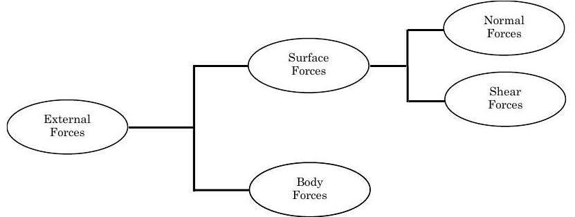
Figure \(\PageIndex{8}\): Classification of External Forces
Transport of linear momentum with force
Experience has shown that the linear momentum of a closed system can only be changed by the application of an external force (This is how Newton originally stated his second law). Thus an external force applied to a closed system must transfer linear momentum between the system and its surroundings. More specifically, \[\mathbf{F}_{\text {external}} \equiv \dot{\mathbf{P}}_{\text {Force}} = \left\{ \begin{array}{c} \text { transport rate of linear momentum } \\ \text { across a boundary due to a force } \end{array} \right\} \nonumber \] where the direction of the momentum flow is in the same direction as the force.
An external force is a mechanism for transferring linear momentum and is a transport rate for linear momentum across the boundary between a system and its surroundings. A force is a vector with all of the properties discussed earlier. The primary dimensions for force are \([\mathrm{M}][\mathrm{L}] /[\mathrm{T}]^{2}\), which are the dimensions of [Linear Momentum]/[Time]. The typical unit for force is a newton \( (\text{N}) \) in SI and a pound-force \( (\text{lbf}) \) in USCS.
When several forces act on a system, the net transport rate of linear momentum into a system with the external forces is written mathematically as below: \[\sum_{j} \mathbf{F}_{\text {ext } j} \equiv \left\{ \begin{array}{c} net \text { transport rate of linear momentum} \\ \text {into the system with force} \end{array}\right\} \nonumber \] External forces, as shown in Figure \(\PageIndex{8}\), can be classified as either surface forces or body forces. Surface forces can be further classified as either normal or shear forces.
Body Forces
A body force always acts in a distributed fashion within the volume of the system and is the result of placing the system in a force field, e.g. a gravitational field, electric field, or magnetic field. Because of this a body force is sometimes called a "force at a distance." Since it acts over the volume of the system, the body force can only be calculated once the system is defined.
The most commonly occurring body force is weight — the force exerted by the Earth on a mass placed in the Earth's gravitational field. Although a body force acts throughout the system, its effect is frequently represented as a concentrated force that acts at a specified point within the system. When the field strength is spatially uniform as it is in the Earth's gravitational field, the weight of an object is assumed to act at the center of gravity of the system. Near the Earth's surface, when an object is suspended from its center of gravity, the object will be perfectly balanced.
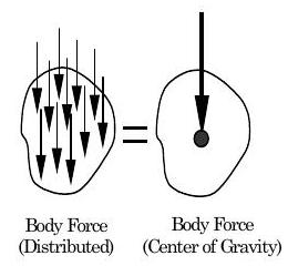
Figure \(\PageIndex{9}\): Body force due to gravity
Determine the magnitude, direction, and point of application of the weight vector for systems A, B, and C. Each system is made of a material with a density of \(900 \mathrm{~kg} / \mathrm{m}^{3}\). In each case, sketch your system and locate the center of gravity. [Hint: You might try your physics book, your calculus or a good mathematics table to find the location of the centroid of these volumes.]
| System A | System B | System C |
|---|---|---|
| Right circular cylinder with diameter \(D = 20 \ \text{cm}\) and height \(H = 40 \ \text{cm}\). |
A right circular cone with diameter \(D = 20 \ \text{cm}\) and height \(H = 40 \ \text{cm}\). |
A hemisphere of diameter \(D = 20 \ \text{cm}\). |
Surface Forces
A surface force is characterized by having a point or points of physical contact on the boundary surface, and for this reason it is sometimes referred to as a contact force. Physically, surface forces always act over a finite area, i.e. they are distributed forces.
Typically, we usually represent the surface forces by a single concentrated force (see Figure \(\PageIndex{10}\)). When a surface force acts on a plane surface and either the area is small or the force is uniformly distributed over the area, it is reasonable to model the distributed force as a single concentrated force with a point of application at the centroid of the area.
.png?revision=1)
Figure \(\PageIndex{10}\): Surface forces
When the surface is curved or the distributed force is non-uniform, a single concentrated force can still be used to model the distributed force; however, the exact point of application must be carefully computed and is not necessarily the centroid of the area over which the distributed force acts.
Every surface force can, if necessary, be further decomposed into two components: a normal and a shear component, as shown in Figure \(\PageIndex{11}\). The line of action of a normal force is perpendicular to the surface at the point of application, and the line of action of a shear force is tangent to the surface at the point of application. Some external forces are by their very nature purely normal or purely shear forces. For example, the force produced by the pressure of the atmosphere on any surface is always a normal force, while the force due to friction is always a shear force.
.png?revision=1)
Figure \(\PageIndex{11}\): Normal and shear forces.
Surface Forces due to Pressure
One of the most ubiquitous forces in our lives is the force of the atmosphere. Because of this we must consider how to determine surface forces due to pressure. By definition, pressure is defined as the force per unit area. The dimensions for pressure are \([\mathrm{F}]/[\mathrm{L}]^2 = \{ [\mathrm{M}][\mathrm{L}]/[\mathrm{T}]^2 \} / [\mathrm{L}]^2 = [\mathrm{M}][\mathrm{L}]^{-1} [\mathrm{T}]^{-2}\). Typical units for pressure are newton per square meter or pascals \((\mathrm{Pa})\) in SI with \(1 \ \text{Pa} = 1 \ \text{N}/\text{m}^2\). In USCS, the units are pounds-force per square inch (\(\text{psi}\) or \(\text{lbf}/\text{in}^2\)) or pounds-force per square foot (\(\text{psf}\) or \(\text{lbf}/\text{ft}^2\)) with \(144 \ \text{psi} = 144 \ \text{lbf}/\text{in}^2 = 1 \ \text{lbf}/\text{ft}^2\).
The standard value of atmospheric pressure on the surface of the earth is \(P_{\text{atm}} = 101325 \ \text{Pa} = 101.325 \ \text{kPa} = 14.696 \ \text{lbf}/\text{in}^2\). These values are frequently rounded off to \(101.3 \ \text{kPa}\) and \(14.7 \text{lbf}/\text{in}^2\).
To evaluate the force due to pressure acting on a surface we must first define the surface (see Figure \(\PageIndex{12}\)). Mathematically, the force is calculated using the integral of the pressure over the surface area as below:
\[ \mathbf{F}_{\text{pressure}} = - \int\limits_{A_{\text{surface}}} \mathbf{n} P \ dA \nonumber \]where \(P\) is the pressure acting on the boundary, \(\mathbf{n}\) is the unit normal vector that points out from the system into the surroundings, and \(dA\) is the differential area over which the pressure acts. Thus, the direction of the pressure force is always into the system.
.jpg?revision=1)
Figure \(\PageIndex{12}\): Geometry for pressure force calculation.
The simplest and also the most common application is one where the pressure is uniform and the surface is flat. Under these conditions Eq. \(\PageIndex{20}\) can be greatly simplified since both the unit normal vector and the pressure come outside the integral:
\[ \begin{align} \mathbf{F}_{\text{pressure}} &= - \int\limits_{A_{\text{surface}}} \mathbf{n} P \ dA \nonumber \\ &= -(\mathbf{n} P) \underbrace{ \int\limits_{A_{\text{surface}}} dA }_{= A_{\text{surface}}} = - P A_{\text{surface}} \mathbf{n} \end{align} \nonumber \]
In words, this says that the pressure force on a flat surface due to a uniform pressure is a vector that is perpendicular to the surface, points into the system, and has a magnitude equal to \(P A_{\text {surface, }}\), the product of the pressure and the surface area. Furthermore, it can be shown (after we study angular momentum) that the point of application of the force is at the centroid of the surface area.
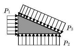
As an example, consider a triangular solid with constant width into the paper as shown in Figure \(\PageIndex{13}\). A uniform pressure acts on each of the three sides as shown in the figure. Since each pressure is uniform and the surfaces are flat the equivalent pressure force vector can be calculated using Eq. \(\PageIndex{21}\). For each side, the force vector points into the surface, is normal to the surface, and has a magnitude equal to the product of the pressure and the surface area over which the uniform pressure acts.
 a) Pressure distributions
.jpg?revision=1) b) Pressure force vectors
b) Pressure force vectorsFrequently, we will have systems that are subjected to atmospheric pressure over the entire system boundary. Imagine for a minute any particular object you would like, say your car or an apple hanging on a string, that is subjected to a uniform atmospheric pressure on all sides. What is the net force of the atmosphere on the object? Based on your experience, I assume you would say the net force due to the atmosphere pressure is zero. You can repeat this experiment and you will find that the net force on any object surrounded by a uniform pressure will be zero regardless of the shape of the object or the value of the pressure.
This leads us to another interesting result. Consider the irregular shaped solid shown in Figure \(\PageIndex{14}\). Imagine that the object is subjected to a uniform pressure on all sides and that the resulting pressure force vectors are shown on the figure. Now we know from experience that if the only forces are due to the uniform pressure then there is no net force on the object due to the pressures. If this were not true, then the object would have a tendency to move (and we would patent this device and retire to the Caribbean). This must mean that the pressure force acting on the left side of the solid must equal the sum of the pressure forces acting over the right side of the solid. As we have shown the pressure force is proportional to surface area. So why doesn't the left side have more pressure force than the right side? The key is in the vector nature of force.
.jpg?revision=1)
Figure \(\PageIndex{14}\): Pressure forces using projected areas.
To help us understand this result, let’s only consider the force in the \(x\)-direction. Now we see that the pressure force acting over the left side of the solid must equal the \(x\)-components of the pressure forces acting on the right side of the solid. Without resorting to complicated mathematics, we can summarize this result as follows:
The magnitude of the pressure force in any direction is equal to the product of the pressure and the projected area in the desired direction.
The projected area is the two-dimensional area observed when the surface is viewed in the direction of interest. Consider a sphere with diameter \(D\) and a cylinder with diameter \(D\) and height \(H\). When observed from any direction, the sphere looks like a circle with projected area \(\pi D^{2} / 4\). Now consider the cylinder. When viewed from either end the cylinder also has a projected area of \(\pi D^{2} / 4\); however, when viewed from the side (perpendicular to its axis of symmetry), the projected area of the cylinder is a rectangle of area \(D H\).
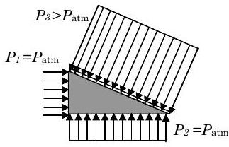
We will also frequently have problems where only a small portion of the system boundary is subjected to non-atmospheric pressure. Under these conditions, we can greatly simplify the pressure force calculations by "subtracting off" atmospheric pressure. Consider the familiar triangular solid as shown in Figure \(\PageIndex{15}\).
.jpg?revision=1)
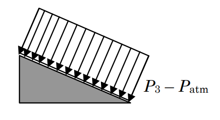.png?revision=1&size=bestfit&width=365&height=199)
c) Resulting pressure distribution with
\(P_{3, \text{new}} = P_3 - P_{\text{atm}}\)
\[ \mathbf{F}_{\text{net}} = - ( P_3 - P_{\text{atm}}) A_3 \mathbf{n} \nonumber \]
For this example, we will assume that all surfaces except one are subjected to atmospheric pressure and this surface has a uniform pressure \(P_{3}>P_{\mathrm{atm}}\). As shown in the figure, we can use the standard integral to evaluate the net force due to the pressures acting on the system. Since the net force due to a uniform atmospheric pressure on all surfaces is zero as shown in part (b) of Figure \(\PageIndex{15}\) we can subtract this zero force from the integral. Once this is done, the integral for net force can be rearranged as shown and we discover that the net force is the result of the pressure measured with respect to atmospheric pressure (this is sometimes referred to as gage pressure). Finally, as shown in part (c) the magnitude of the net force is just \(\left(P_{3}-P_{\text {atm}}\right) A_{3}\). Since \(P_{3}>P_{\text {atm}}\), the force arrow points into surface 3. When some portion of a system's boundary is subjected to non-atmospheric pressure, subtracting out the atmospheric pressure will greatly simplify the calculation of the net pressure force.
To give us some quick practice with these ideas, consider the plumber's helper used to unclog toilets. The classic plumber's helper consists of a hollow rubber hemisphere attached to a wooden stick. The rubber material is flexible and will deform when pushed against a surface. If applied to a smooth surface, as shown in the figure, the air will be squeezed out of the hemisphere. This lowers the pressure inside the deformed hemisphere and causes the plumber's helper to "stick" to the surface. What exactly is the net force in the vertical direction due to pressure on the plumber's helper?
.png?revision=2&size=bestfit&width=377&height=666)
Figure \(\PageIndex{16}\): The plumber's helper.
Solution
Consider the system shown above by the dashed lines. The cup in contact with the surface is of diameter \(D\). The pressure on every surface of the system except the open end of the rubber cup (top surface) is subjected to atmospheric pressure, \(P_{\text{atm}}\). The surface that covers the open end of the cup sees a pressure \(P_{\text{cup}}\)—the pressure of the air trapped inside the deformed hemisphere.
The projected area of the plumber's helper, when viewed from the top or bottom along the vertical direction, is just a circle with area \((\pi / 4) D^{2}\). Also, since we want to find the net force we can just subtract out the atmospheric pressure.
Thus
\[ \begin{align*} & \mathbf{F}_{\text {net pressure}} = -\left(P_{\text {cup}} - P_{\text {atm}}\right) A_{\text {projected}} \mathbf{n} \\ \uparrow+ & F_{\text {net pressure}} = -\left(P_{\text {cup}} - P_{\text {atm}}\right) \left(\frac{\pi}{4} D^{2}\right)(1)=\left(P_{\text {atm}} - P_{\text {cup}}\right) \left(\frac{\pi}{4} D^{2}\right) \\ & \mathbf{F}_{\text {net pressure}} = \left(P_{\text {atm}}-P_{\text {cup}}\right) \left(\frac{\pi}{4} D^{2}\right) \angle 90^{\circ} \quad \text { or } \quad \left(P_{\text {atm}}-P_{\text {cup}}\right) \left(\frac{\pi}{4} D^{2}\right) \uparrow \end{align*} \nonumber \]
As you might expect if \(P_{\text {cup}}<P_{\text {atm}\), the net force will be up (in the positive \(y\)-direction). There are at least two other forces acting on this system that will govern whether it "sticks" or falls—the weight of the system and the force of the smooth surface on the system where it contacts the rubber hemisphere.
Linear momentum transport with mass flow
As was shown earlier, every lump of mass with a velocity has linear momentum. When mass is allowed to flow across the boundary of an open system, each lump of mass carries with it linear momentum. Thus the linear momentum of an open system can also be changed by mass flow carrying linear momentum across the system boundary. The rate at which linear momentum is transported across the boundary can be represented by the product of the mass flow rate and the local velocity at the boundary, assuming that the velocity is uniform: \[\dot{\mathbf{P}}_{\text {mass}} = \dot{m} \mathbf{V} = \left\{\begin{array}{c} \text { transport rate of linear momentum } \\ \text { with mass flow } \end{array}\right\} \nonumber \] where \(\dot{m}\) is the mass flow rate at the flow boundary where the velocity \(\mathbf{V}\) is uniform. The dimension for this quantity is \([\mathrm{M}][\mathrm{L}] /[\mathrm{T}]^{2}\).
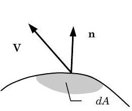
Figure \(\PageIndex{17}\): Mass transport of linear momentum at a boundary.
For conditions where the velocity is not spatially uniform at the flow boundary, the linear momentum transport rate must be calculated from using an integral. At any flow boundary as shown in Figure \(\PageIndex{17}\), the transport of linear momentum out of the system can be characterized by the integral: \[\begin{array} \dot{\mathbf{P}}_{\text {mass, out}} &= \displaystyle \int\limits_{A_{\text {sys}}}(\mathbf{V}) \left( \rho \mathbf{V}_{\text {rel}} \cdot \mathbf{n} \right) \ dA \\ &= \displaystyle \int\limits_{A_{\text {sys}}}(\mathbf{V}) \left(\rho V_{\text {n, rel}}\right) \ dA \end{array} \nonumber \] where \(\mathbf{V}\) is the local velocity vector measured with respect to an inertial reference frame, \(\mathbf{V}_{\text{rel}}\) is the local velocity vector measured with respect to the surface, \(\mathbf{n}\) is the unit vector normal to the differential surface area \(d A\) and points out from the system, and \(V_{\text{n, rel}} = \mathbf{V}_{\text {rel}} \cdot \mathbf{n}\), the magnitude of the normal component of the velocity \(\mathbf{V}_{\text {rel}}\).
If the velocity is spatially uniform at the flow cross section, the mass transport of linear momentum can be written in terms of the mass flow rate at the boundary and the velocity as follows:
\[ \begin{align} \dot{\mathbf{P}}_{\text{mass, out}} &= \int\limits_{A_{\text{sys}}} (\mathbf{V}) \left( \rho V_{\text{n, rel}} \right) \ dA = (\mathbf{V}) \left( \rho V_{\text{n, rel}} \right) \int\limits_{A_{\text{sys}}} dA \nonumber \\[4pt] &= (\mathbf{V}) \left( \rho V_{\text{n, rel}} \right) A_{\text{sys}} = \left( \rho V_{\text{n, rel}} A_{\text{sys}} \right) \mathbf{V} \\ &= \dot{m}_{\text{out}} \mathbf{V} \nonumber \end{align} \nonumber \]
This is often referred to as one-dimensional flow. If the velocity is not uniform across the flow area, the flow area must be broken into a suitable number of areas where the velocity can be assumed uniform and Eq. \(\PageIndex{24}\) will become a summation. Alternatively, the non-uniform velocity distribution can be handled by performing the integral in Eq. \(\PageIndex{23}\).
The net transport of linear momentum with mass flow rate can be obtained by summing up the transports at all flow boundaries: \[\sum_{\text {in}} \dot{m}_{i} \mathbf{V}_{i} - \sum_{\text {out}} \dot{m}_{e} \mathbf{V}_{e} \equiv \left\{ \begin{array}{c} net \text { transport rate of linear momentum } \\ into \text { the system with mass flow } \end{array}\right\} \nonumber \] Notice that the net transport may be positive or negative depending upon the relative transports.
5.1.4 How can linear momentum be generated or destroyed in a system?
Experience has shown that the linear momentum of a system cannot be created or destroyed. Recognizing that linear momentum is an extensive property, we can state this law as follows:
Linear momentum is a conserved property.
Once again you are reminded that the use of the word "conservation" is different in this course (ES201) than you are familiar with in physics. (C'mon, take at look at your physics book and see what kind of problems they solve in the section labeled "conservation of linear momentum." Do the problems involving conservation of energy differ from the problems involving conservation of linear momentum?) In this course, when we say that something is conserved we are making a general statement about the way the world behaves and not a problem specific modeling assumption. In fact, you could say that it is incorrect (if not redundant) to write in a problem solution "assume that linear momentum (or mass or charge) is conserved." You can't invoke basic physical laws by assuming their existence. It would be correct to say "using (or applying) the conservation of linear momentum (or mass or charge) we find that..." The basic physical laws apply whether we want them to or not.
5.1.5 Putting it all together!
Using the accounting framework, we can now develop the following statement for conservation of linear momentum: \[\left[ \begin{array}{c} \text { Rate of accumulation } \\ \text { of } \\ \text { linear momentum } \\ \text { inside a system } \\ \text { at time } t \ \end{array} \right] = \left[ \begin{array}{c} \text { Net transport rate of } \\ \text { linear momentum } \\ \text { into the system } \\ \text { by external forces } \\ \text { at time } t \ \end{array}\right] + \left[\begin{array}{c} \text { Net transport rate of } \\ \text { linear momentum } \\ \text { into the system } \\ \text { by mass flow } \\ \text { at time } t \ \end{array}\right] \nonumber \] or in symbols, conservation of linear momentum (rate form) becomes \[\frac{d \mathbf{P}_{\text {sys}}}{d t} = \sum \dot{\mathbf{P}}_{\text {force}} + \sum_{\text {in}} \dot{\mathbf{P}}_{\text {mass, in}} - \sum_{\text{out}} \dot{\mathbf{P}}_{\text {mass, out}} \nonumber \]
Using the more familiar symbols of forces, mass flow rates, and specific linear momentum, the rate form of the conservation of linear momentum becomes \[\frac{d \mathbf{P}_{\mathrm{sys}}}{d t} = \sum \mathbf{F}_{\text {ext}} + \sum_{\text {in}} \dot{m}_{i} \mathbf{V}_{i} - \sum_{\text {out}} \dot{m}_{e} \mathbf{V}_{e} \label{RateFormLN} \] In words we might say the following:
The time rate of change of the linear momentum of the system equals the net transport rate of linear momentum into the system by external forces plus the net transport rate of linear momentum into the system by mass flow.
Under some conditions, the integrated or finite-time form is useful. In words, the finite-time form of the conservation of linear momentum is \[ \left[ \begin{array}{c} \text { Linear } \\ \text { momentum } \\ \text { inside the } \\ \text { system at } \\ \text { time } t_{2} \end{array}\right] - \left[\begin{array}{c} \text { Linear } \\ \text { momentum } \\ \text { inside the } \\ \text { system at } \\ \text { time } t_{1} \end{array}\right] = \left[\begin{array}{c} \text { Net transport of } \\ \text { linear momentum } \\ \text { into the system } \\ \text { by external forces } \\ \text { during the period } \Delta t \end{array}\right]+\left[\begin{array}{c} \text { Net transport of } \\ \text { linear momentum } \\ \text { into the system } \\ \text { by mass flow } \\ \text { during the period } \Delta t \end{array}\right] \nonumber \]
or in equation form, \[\Delta \mathbf{P}_{\mathrm{sys}} = \sum_{\text {external}} \left( \int\limits_{t_{1}}^{t_{2}} \mathbf{F} \ dt \right) + \sum_{\text {in}} \left( \int\limits_{t_{1}}^{t_{2}} \left(\dot{m}_{i} \mathbf{V}_{i}\right) \ d t \right) - \sum_{\text {out}} \left(\int\limits_{t_{1}}^{t_{2}} \left(\dot{m}_{e} \mathbf{V}_{e}\right) \ dt \right) \nonumber \] Although this last form of the conservation of linear momentum equation looks rather complicated, it is really much simpler to focus on the rate form and then, if necessary, perform the required integration to recover Equation \(\PageIndex{30}\).
Newton's Laws are commonly written as follows:
Law I: If the resultant force acting on a particle is zero, the particle will remain at rest (if originally at rest) or will move with constant speed in a straight line (if originally in motion)
Law II: If the resultant force acting on a particle is not zero, the particle will have an acceleration proportional to the magnitude of the resultant force and in the direction of this resultant force
Law III: The forces of action and reaction between bodies in contact have the same magnitude, same line of action, and opposite sense.
Demonstrate that these three laws are satisfied by the application of the rate-form of the Conservation of Linear Momentum.
Solution
Known: Newton's three laws of mechanics
Find: Show that these laws are supported by the conservation of linear momentum
Given: Provided as needed.
Analysis:
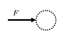
Newton's First Law: Look at a single particle as shown in the figure. To apply the conservation of linear momentum, we select the particle as a system and sketch a linear momentum interaction (free-body) diagram for the body.
.png?revision=1)
Figure \(\PageIndex{18}\): A system consisting of a particle. Free-body diagram of this system, which has no interactions with its surroundings.
Writing the rate-form of the conservation of linear momentum for this system we have:
\[ \begin{align*} &\frac{d \mathbf{P}_{\text{sys}}}{dt} = \underbrace{ \cancel{ \sum \mathbf{F}_{\text{ext}} } }_{ \begin{array}{c} =0 \text{ because there} \\ \text{are no external} \\ \text{forces} \end{array} } + \underbrace{ \cancel{ \sum_{\text{in}} \dot{m}_i \mathbf{V}_i - \sum_{\text{out}} \dot{m}_e \mathbf{V}_e } }_{\begin{array}{c} =0 \text{ because} \\ \text{it is a closed system} \end{array} } \\ &\frac{d \mathbf{P}_{\text{sys}}}{dt} = 0 \quad \rightarrow \quad 0 = \frac{d \mathbf{P}_{\text{sys}}}{dt} = \frac{ d (m \mathbf{V})}{dt} = m \frac{d \mathbf{V}}{dt} \end{align*} \nonumber \]
Thus, \(\dfrac{d \mathbf{V}}{dt} = 0\) and \(\mathbf{V}\) is a constant!
This demonstrates that with no transports of linear momentum by force, i.e. with no external forces acting on the particle, the velocity of the particle remains constant.
Newton's Second Law: The system is the same as before, only this time there is a force acting on the system.
.png?revision=1)
Figure \(\PageIndex{19}\): Free-body diagram of a system consisting of a particle with a force acting on it.
\[ \begin{align*} &\frac{d \text{P}_{\mathrm{sys}}}{dt} = \mathbf{F} + \underbrace{ \cancel{ \sum_{\text {in}} \dot{m}_{i} \mathbf{V}_{i} - \sum_{\text {out}} \dot{m}_{e} \mathbf{V}_{e} } }_{\begin{array}{c} =0 \text { because } \\ \text { it is a closed system } \end{array} } \\ &\frac{d \mathbf{P}_{\text {sys}}}{d t} = \mathbf{F} \quad \rightarrow \quad \mathbf{F} = \frac{d \mathbf{P}_{\text {sys}}}{d t} = \frac{d(m \mathbf{V})}{d t} = m \underbrace{\frac{d \mathbf{V}}{d t}}_{= \mathbf{a}} = m \mathbf{a} \end{align*} \nonumber \]
Thus \(\mathbf{F}=m \mathbf{a}\) and \(\mathbf{a}=\mathbf{F} / m\).
This demonstrates that the acceleration vector is proportional to the external force vector, so the magnitude of the acceleration is proportional to the applied force and the direction is the same as the direction of the applied force.
Newton's Third Law: This time our system is the interface or the contact surface between two particles that are in contact. This interface as shown in the drawing below has no mass inside it and is acted on by two forces - \(\mathbf{F}_{\mathrm{A-B}}\), the force of particle \(\mathrm{A}\) on particle \(\mathrm{B}\), and \(\mathbf{F}_{\mathrm{B-A}}\), the force of particle \(\mathrm{B}\) on particle \(\mathrm{A}\).
.png?revision=1)
Figure \(\PageIndex{20}\): System consisting of the contact interface between two particles.
Writing the conservation of linear momentum equation for this system gives the following:
\[ \begin{align*} \underbrace{ \cancel{ \frac{d \mathbf{P}_{\text{sys}}}{dt} } }_{\begin{array}{c} =0 \text{ because the system} \\ \text{has no mass, so } \mathbf{P} = 0 \\ \text{for all time.} \end{array} } = \mathbf{F}_{\text{A-B}} + \mathbf{F}_{\text{B-A}} + \underbrace{ \cancel{ \sum_{\text{in}} \dot{m}_i \mathbf{V}_i - \sum_{\text{out}} \dot{m}_e \mathbf{V}_e } }_{\begin{array}{c} =0 \text{ because} \\ \text{it is a closed system} \end{array}} \\ 0 = \mathbf{F}_{\text{A-B}} + \mathbf{F}_{\text{B-A}} \quad \rightarrow \quad \mathbf{F}_{\text{B-A}} = -\mathbf{F}_{\text{A-B}} \end{align*} \nonumber \]
Thus, the forces of action and reaction at a point of contact between two systems are vectors of equal magnitude, opposite sign, and the same line of action.
Comment: The important point here is that all three of Newton's laws of mechanics are incorporated into the Conservation of Linear Momentum principle as formulated here.