7.8: Electrical Energy Storage and Transfer

Because of its importance and its uniqueness, we need to take a closer look at the transfer and storage of electrical energy. As a start, what exactly do we mean by electrical energy? For our purposes, we will define electrical energy as the energy that is stored in an electric or a magnetic field. Our emphasis here will be to consider how the conservation of energy principle applies to devices and systems commonly found in electrical and electronic devices. We will limit ourselves to systems that can be modeled using lumped circuit elements (as discussed in Section 4.3 of Chapter 4).

7.8.1 Instantaneous and Average Power

Earlier in this chapter, we developed an equation for the electric power in terms of the flow of an electric current through the system and the electric potential difference at the terminals where the current enters and leaves the system. In our earlier development, we tacitly assumed that the current and voltages were independent of time. In reality, we know that almost all of our electric power is supplied in the form of a time-varying alternating current. The transient behavior of electrical circuits is also of interest in the design of everything from power systems to control systems to computers. In this section, we will address the problem of calculating AC power.

Figure \(\PageIndex{1}\): Two-terminal system for electric work and power.

Instantaneous Electric Power

For purposes of our discussion, we will restrict ourselves to a two-terminal system as shown in Figure \(\PageIndex{1}\). The electric current \(i\) flows into the system at a terminal with voltage \(V_{\text {in-o}}\) and leaves the system at a terminal with voltage \(V_{\text {out-o}}\). Both voltages are measured with respect to the same ground point (point \(O\)). In addition, we will assume that the voltages and current may change with time. Under these conditions, our earlier expression for electric power is still valid; but it represents the instantaneous electric power for a system: \[\begin{array}{ll} \dot{W}_{\text {electric, in}} & =i \cdot\left(V_{\text {in-o}}-V_{\text {out-o}}\right) \quad & \\ &= i \cdot \Delta V & \text { Instantaneous Electric Power } \end{array} \nonumber \] By convention, the instantaneous electric power is positive when the current enters the system at the terminal with the higher voltage and negative when it leaves the system at the terminal with the higher voltage.

In a DC (direct-current) system, the instantaneous power is a constant and independent of time; thus, the instantaneous electric power is also constant and independent of time.

In an AC (alternating-current) system, the current \(i\) and the voltage difference \(\Delta V\) for the terminals can be described as sinusoidal functions of time: \[\Delta V=V_{\max } \cos (\omega t) \quad \text { and } \quad i = i_{\max } \cos (\omega t+\theta) \nonumber \] where \(\omega\) is the frequency \((\mathrm{rad} / \mathrm{s})\), \(t\) is the time \((\mathrm{s})\), and \(\theta\) is the phase angle (radians) that describes how current leads or lags the voltage \([-\pi / 2 \leq \theta \leq \pi / 2]\). The period for one cycle depends on the frequency as follows: \[2 \pi=\omega \cdot t_{\text {period}} \quad \rightarrow \quad t_{\text {period}}=\frac{2 \pi}{\omega} \nonumber \]

Under these conditions, the instantaneous power is calculated as follows: \[\begin{array}{l} \dot{W}_{\text {electric, in}} &= i \cdot \Delta V = \left[i_{\max } \cos (\omega t)\right] \cdot\left[V_{\max } \cos (\omega t+\theta)\right] \\ &=i_{\max } \cdot V_{\max } \cdot \cos (\omega t) \cdot \cos (\omega t+\theta) \\ &=i_{\max } \cdot V_{\max } \cdot \dfrac{1}{2} \cdot[\cos (2 \omega t+\theta)+\cos (\theta)] \end{array} \nonumber \] where the last line is obtained by applying a standard trigonometric relationship for multiplying cosines. Before leaving this expression it is helpful to separate the instantaneous power, Eq. \(\PageIndex{4}\), into two parts: \[\begin{array}{l} \dot{W}_{\text {electric, in}} &= i_{\max } \cdot V_{\max } \cdot \dfrac{1}{2} \cdot [\cos (2 \omega t+\theta)+\cos (\theta)] \\ &=\underbrace{\dfrac{i_{\max } \cdot V_{\max }}{2} \cos (\theta)}_{\begin{array}{c} \text {Time-independent} \\ \text{component} \end{array}} + \underbrace{\dfrac{i_{\max } \cdot V_{\max }}{2} \cos (2 \omega t+\theta)}_{\begin{array}{c} \text{Time-varying periodic} \\ \text{component} \end{array}} \end{array} \nonumber \] The first part is independent of time and only depends on the phase angle, \(\theta\), while the second component varies periodically with time. A careful examination of Eq. \(\PageIndex{5}\) shows that the instantaneous AC power is a sinusoidal function that oscillates between zero and a maximum (or peak) value of \(i_{\max} \cdot V_{\max} \cdot \cos(\theta)\).

Average Electric Power

The average electric power is defined as the amount of electric energy transferred across a boundary divided by the time interval over which the transfer occurs. Mathematically, the average electric power for a time interval \(t_{\mathrm{obs}}\) can be calculated from the equation \[\dot{W}_{\text {avg, in}} = \frac{1}{t_{\text {obs}}} \int\limits_{0}^{t_{\text {obs}}} \dot{W}_{\text {electric, in}} \ dt \nonumber \] If the voltage and current are constants as they would be in a DC system, the average power and the instantaneous power are identical. In an AC system, the average power would be calculated over the time period for one cycle of the instantaneous power (or two cycles of the voltage and current) as follows: \[\begin{aligned} \dot{W}_{\text {avg, in}} &= \frac{1}{t_{\text {obs}}} \int\limits_{0}^{t_{\text {obs}}} \dot{W}_{\text {electric, in}} \ dt \quad \text { where } \quad\quad\quad t_{\text {obs}}=t_{\text {period}}=\frac{2 \pi}{2 \omega}=\frac{\pi}{\omega} \\ &=\frac{1}{t_{\text {period}}} \int\limits_{0}^{t_{\text {period}}}\left[\frac{i_{\max } \cdot V_{\max }}{2} \cos (\theta)\right] dt \quad\quad\quad \left| \begin{array}{l} \text { What happened to the } \\ \text { time-varying component? } \end{array} \right. \\ &=\frac{1}{t_{\text {period}}}\left[\frac{i_{\max } \cdot V_{\max }}{2} \cos (\theta)\right] t_{\text {period}} = \frac{i_{\max } \cdot V_{\max }}{2} \cos (\theta) \end{aligned} \nonumber \]

This finally gives \[\dot{W}_{\text {avg, in}} = \frac{1}{2} i_{\max } \cdot V_{\max } \cdot \cos (\theta) \quad\quad\quad \begin{array}{c} \text {Average} \\ \text{AC electric power} \end{array} \nonumber \] Thus the average power can be calculated knowing the maximum (or peak) values for current voltage and the angle \(\theta\). Note, that the numerical constant of \(1 / 2\) depends on the shape of the voltage and current signals and not the specific frequency. If the voltage and current signals had a different shape, such as a sawtooth wave or a square wave, the numerical constant would change.

7.8.2 AC Power and Effective Voltage and Current

What exactly do we mean when we say 110 ac volts? Is this the maximum (or peak) voltage? Is it the average? But the average wouldn't make any sense because the average of a sinusoid that oscillates around zero is zero. It may seem strange to you, but there once was a time when electric power was distributed using DC voltages and currents. Unfortunately for Thomas Edison, who promoted DC distribution, AC systems won out. However, the ghost of DC still lives in the way we talk about AC voltages and currents. It turns out that AC voltage and current are reported in terms of their effective values that are related to a DC equivalent that would deliver the same average power to a resistor.

The effective value of an AC current \(i_{\text {eff}}\) equals the value of a DC current that would deliver the same average power to a load resistor. The relationship between the maximum AC current and the effective value of the AC current is developed below.

\[ \begin{aligned} \left. \dot{W}_{\text{electric, in}} \right|_{average, \ DC} \ &= \ \left. \dot{W}_{\text{electric, in}} \right|_{average, \ AC} \\ i_{\text{eff}}{ }^{2} \cancel{ R_{\text{load}} } &= \frac{1}{t_{\text{period}}} \int\limits_{0}^{t_{\text{period}}} i^2 \cancel{ R_{\text{load}} } \ dt = \frac{1}{t_{\text{period}}} \int\limits_{0}^{t_{\text{period}}} \left[i_{\max} \cos (\omega t + \theta) \right]^{2} \cancel{ R_{\text{load}} } \ dt \end{aligned} \nonumber \]

\[\begin{aligned} i_{\text {eff}}{ }^{2} &= i_{\max }{ }^{2} \left\{\frac{1}{t_{\text {period}}} \int\limits_{0}^{t_{\text {period}}} [\cos (\omega t+\theta)]^{2} \ dt\right\} \\ &=i_{\max }{ }^{2} \left\{\frac{1}{t_{\text {period}}} \int\limits_{0}^{t_{\text {period}}} \left[\frac{1}{2}+\frac{1}{2} \cos (2 \omega t+2 \theta)\right] \ dt \right\} \\ &=\left\{\frac{1}{t_{\text {period}}} \left[\frac{1}{2}\left(t_{\text {period}}-0\right)+0\right]\right\}^{2} = \frac{i_{\max }{ }^{2}}{2} \end{aligned} \nonumber \] Thus we have the final result: \[i_{\text {eff}} = \frac{i_{\max }}{\sqrt{2}} \quad \text { Effective AC current } \nonumber \]

If the time-varying current had a different waveform than a sinusoid, say a square wave or a sawtooth wave, the constant in the numerator would take on a different value.

Similarly, the effective value of an AC voltage \(V_{\text {eff}}\) equals the value of a DC voltage that would deliver the same average power to a load resistor. Using a development similar to the one for effective current, we discover that: \[V_{\text {eff}} = \frac{V_{\max }}{\sqrt{2}} \quad \text { Effective AC voltage } \nonumber \] And this is the answer to the question we started out with — what is a \(110 \mathrm{AC}\) voltage? The 110 volts is the effective value of the \(\mathrm{AC}\) voltage. So on an oscilloscope, a 110-AC-volt signal would be a sinusoid with a maximum value \(V_{\max }=110 \cdot \sqrt{2}=155.6\) volts. A 220-AC-volt signal would have a maximum value of \(311.1\) volts.

Now if we revisit the equation for the average AC power, we can rewrite it in terms of the effective values: \[\begin{array}{l} \dot{W}_{\text {avg, in}} &=\dfrac{i_{\max } \cdot V_{\max }}{2} \cos (\theta) = \left(\dfrac{i_{\max }}{\sqrt{2}}\right)\left(\dfrac{V_{\max }}{\sqrt{2}}\right) \cos (\theta) \\ { } \\ &=\underbrace{i_{\text {eff}} \cdot V_{\text {eff}}}_{\begin{array}{c} \text{Apparent} \\ \text{Power} \end{array}} \cdot \underbrace{\cos (\theta)}_{\begin{array}{c} \text{Power} \\ \text{Factor} \end{array}} \quad\quad\quad\quad {\text {Average AC Power }} \end{array} \nonumber \] Thus the average AC power transferred at a system boundary is the product of the effective current, the effective voltage, and \(\cos (\theta)\).

A closer examination of the average AC power relation, Eq. \(\PageIndex{10}\), shows that it is the product of the apparent power and the power factor. Because the apparent power is not really a power, it is frequently given the units of volt-amps. (If you look on the nameplate on heavy duty electrical equipment you will frequently see values reported in \(\mathrm{kV} \cdot \mathrm{A}\), kilovolt-amps.) The power factor can have a value between \(0\) and \(1\) and depends on the behavior of the load, specifically the load impedance. Determining the phase angle and power factor for a specific electrical system is the subject of courses in circuit analysis, e.g. ES203 — Electrical Systems, which most of you will be taking later. For systems with a purely resistive load the power factor is one \([\theta=0\) and \(\cos (\theta)=1]\). In this text, unless you are told differently, you may assume that the power factor is unity. (Note that this assumption always gives you the maximum possible electric power for a given situation.)

7.8.3 Storage of Electrical Energy

When energy is transferred to or from a system by the flow of electrical current, what happens to this energy inside the system? The answer to this question depends on what is inside the system. In this section, we will limit ourselves to devices commonly found in electrical circuits: resistors, capacitors, inductors, and batteries.

For our discussion, we will assume that our system can store energy in six different forms: \[E_{\text {system}} = U + \underbrace{E_{MF}+E_{EF}}_{\text {Electrical Energy}} + \underbrace{E_{K, \text { trans}} + E_{K, \text { rot}} + E_{GP}}_{\text {Mechanical Energy}} \nonumber \] \[\begin{aligned} \text{where} \quad\quad\quad & \\ U &=\text { internal energy } \\ E_{EF} &=\text { energy stored in an electric field } \\ E_{MF} &=\text { energy stored in a magnetic field } \\ E_{K, \text { trans}} &=\text { translational kinetic energy } \\ E_{K, \text { rot}} &=\text { rotational kinetic energy } \\ E_{GP} &=\text { gravitational potential energy } \end{aligned} \nonumber \]

The new players in this discussion are the energy stored in an electric field and the energy stored in a magnetic field. In writing Eq. \(\PageIndex{11}\) with six discrete energy terms, we have assumed that the energy terms are independent of each other. This will be sufficient for our discussion here; however, a more detailed presentation of thermodynamics would reveal that there are many situations where the electrical and internal energy terms are not independent and must be treated as a single term (J. Kestin, A Course in Thermodynamics, Blaisdell Publishing Co, Waltham, Massachusetts, 1966, Chpt 8.).

If we restrict ourselves to a closed system, then the energy balance becomes \[\frac{d}{dt}\left[U + E_{K, \text { trans}} + E_{K, \text { rot}} + E_{GP} + E_{EF}+E_{MF}\right] = \dot{Q}_{\text {net}, \text { in }} + \dot{W}_{\text {net}, \text { in}} \nonumber \] Now let's consider several different components that are often found in an electrical system.

Resistor

One of the most basic components of an electric circuit is a resistor. For our purposes, we will assume that an ideal resistor is one that satisfies Ohm's law \(V_{R}=i R\) as illustrated in Figure \(\PageIndex{2}\) and cannot store energy in electric and magnetic fields.

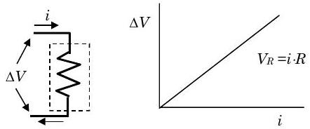
Figure \(\PageIndex{2}\): Voltage-current relationship for an ideal resistor.

If we apply the conservation of energy to an adiabatic, ideal resistor we find the following: \[\begin{aligned} \frac{d}{dt} E_{\text {resistor}} &= \dot{W}_{\text {net, in}} + \cancel{\dot{Q}_{\text {net, in}}}^{=0} \\ \frac{d}{dt} \left[U + \cancel{E_{K, \text { trans}}} + \cancel{E_{K, \text { rot}}} + \cancel{E_{\text {GP}}} + \cancel{E_{\text {MF}}} + \cancel{E_{EF}} \right] &= i \cdot \Delta V \quad \text { where } \Delta V=V_{R} \\ \frac{dU}{dt} &= i \cdot V_{R} = i \cdot(iR) \end{aligned} \nonumber \] Finally we have \[\frac{d E_{\text {resistor}}}{dt} = \frac{dU}{d }=i^{2} \cdot R \nonumber \] So electric power supplied to an adiabatic, ideal resistor results in an increase in the internal energy of the system. For a finite time period, the change in energy of the resistor is \[\Delta E_{\text {resistor}}=\Delta U=\int\limits_{t_{1}}^{t_{2}}\left(i^{2} \cdot R\right) dt \quad \geq 0 \nonumber \] Note that this is an irreversible transfer of energy because changing the direction of the current will not decrease the internal energy of the system.

Capacitor

The second basic circuit component we will examine is the capacitor. A capacitor consists of two charged surfaces separated by a dielectric. For our purposes, an ideal capacitor will be one that can only store energy in an electric field within the capacitor and that satisfies the voltage-current relationship embodied in Figure \(\PageIndex{3}\).

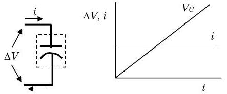
Figure \(\PageIndex{3}\): Voltage-current relationship for an ideal capacitor.

Analysis of this figure shows that the voltage across the capacitor and the current are related by the expression: \[i=C \frac{dV_{C}}{d t} \nonumber \] where \(C\) is the capacitance and is measured in farads \((\mathrm{F})\) and \(1 \mathrm{~F} = (1 \mathrm{~A})(1 \mathrm{~s}) /(1 \mathrm{~V})\).

Applying the conservation of energy to an adiabatic, ideal capacitor gives the following: \[\begin{aligned} \frac{d}{dt} E_{\text {capacitor}} &= \dot{W}_{\text {net, in}} + \cancel{\dot{Q}_{\text {net, in}}}^{= 0} \\ \frac{d}{dt}\left[\cancel{U} + \cancel{E_{K, \text { trans}}} + \cancel{E_{K, \text { rot}}} + \cancel{E_{GP}} + E_{EF} + \cancel{E_{MF}} \right] &= i \cdot \Delta V \quad \text { where } \Delta V=V_{C} \\ \frac{d E_{EF}}{dt} &= i \cdot V_{C} = \left(C \frac{d V_{C}}{dt}\right) \cdot V_{C} \end{aligned} \nonumber \]

Finally we have \[\frac{d E_{\text {capacitor}}}{dt}=\frac{d E_{E F}}{d t}=\frac{d}{d t}\left(C \frac{V_{C}{ }^{2}}{2}\right) \quad \text { where } E_{\text {capacitor }} \equiv C \frac{V_{C}{ }^{2}}{2} \nonumber \] So the instantaneous electric power supplied to an adiabatic, ideal capacitor results in a change in the energy stored in the electric field within the capacitor. If the capacitor is subjected to an AC voltage, the time-averaged energy stored in the capacitor is calculated by substituting the effective voltage as follows. \[\left.E_{\text {capacitor}}\right|_{\text {average AC }} = C \frac{V_{C, \text { eff}}{ }^{2}}{2} \quad\quad \begin{gathered} \text { Average energy stored } \\ \text { in a capacitor driven by } \\ \text { an AC voltage. } \end{gathered} \nonumber \] For a finite-time period, the change in the energy of the capacitor is just the change in the energy of the capacitor: \[\Delta E_{\text {capacitor}} = \Delta E_{EF} = \frac{C}{2}\left(V_{C, 2}{ }^{2}-V_{C, 1}{ }^{2}\right) \nonumber \] Notice that unlike the energy storage in the resistor, the energy stored in an adiabatic capacitor can both increase and decrease.

Inductor

The third basic circuit component we will examine is the inductor. An inductor consists of cylindrical coil of wire. For our purposes, an ideal inductor will be one that can only store energy in a magnetic field within the inductor and that satisfies the voltage-current relationship embodied in Figure \(\PageIndex{4}\).

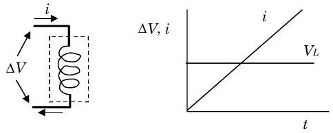
Figure \(\PageIndex{4}\): Voltage-current relationship for an ideal inductor.

Analysis of this figure shows that the voltage across the inductor and the current are related by the expression: \[V_{L}=L \frac{di}{dt} \nonumber \] where \(L\) is the inductance and is measured in henrys \((\mathrm{H})\) and \(1 \mathrm{H} = (1 \mathrm{~V})(1 \mathrm{~s}) / (1 \mathrm{~A})\).

Applying the conservation of energy to an adiabatic, ideal inductor gives the following results: \[\begin{aligned} \frac{d}{dt} E_{\text {inductor}} &= \dot{W}_{\text {net, in}} + \cancel{\dot{Q}_{\text {net, in}}}^{= 0} \\ \frac{d}{dt}\left[\cancel{U} + \cancel{E_{\text {K, trans}}} + \cancel{E_{K, \text { rot}}} + \cancel{E_{GP}} + \cancel{E_{EF}} + E_{MF}\right] &= i \cdot \Delta V \quad \text { where } \Delta V=V_{L} \\ \frac{d E_{MF}}{dt} &= i \cdot V_{L} = i \cdot\left(L \frac{di}{dt}\right) \end{aligned} \nonumber \]

Finally we have \[\frac{d E_{\text {Inductor}}}{dt} = \frac{d E_{MF}}{dt} = \frac{d}{dt}\left(L \frac{i^{2}}{2}\right) \quad \text { where } \quad E_{\text {Inductor}} \equiv L \frac{i^{2}}{2} \nonumber \] So the electric power supplied to an adiabatic, ideal inductor results in a change in the energy stored in the magnetic field within the inductor. If the inductor is subjected to an AC current, the time-averaged energy stored in the energy is calculated by substituting the effective current as follows: \[\left.E_{\text {inductor}}\right|_{AC} = L \frac{i_{\text {eff}}{ }^{2}}{2} \quad\quad \begin{gathered} \text { Average energy stored } \\ \text { in an inductor driven } \\ \text { by an AC current } \end{gathered} \nonumber \] For a finite-time period, the change in the energy of the inductor is just the change in the energy of the inductor: \[\Delta E_{\text {inductor}} = \Delta E_{MF} = \frac{L}{2}\left(i_{2}{ }^{2} - i_{1}{ }^{2}\right) \nonumber \] Notice that unlike the energy stored in the resistor, the energy stored in the adiabatic inductor can both increase and decrease.

Battery

The last component we will consider is the battery. An ideal battery will satisfy the voltage-current relationship shown in Figure \(\PageIndex{5}\) and cannot store energy in electric and magnetic fields.

Figure \(\PageIndex{5}\): Voltage-current relationship for an ideal battery.

If we apply conservation of energy to the adiabatic, ideal battery we have the result that \[\begin{aligned} \frac{d E_{\text {battery}}}{dt} &=\dot{W}_{\text {net, in}} + \cancel{ \dot{Q}_{\text {net, in}} }^{=0} \\ \frac{d}{dt}\left[U + \cancel{E_{K, \text { trans}}} + \cancel{E_{K, \text { rot}}} + \cancel{E_{GP}} + \cancel{E_{UF}} + \cancel{E_{EF}}\right] &= i \cdot \Delta V \quad\quad \text { where } \Delta V=\Delta V_{\text {cell}} \\ \frac{dU}{dt} &= i \cdot \Delta V_{\text {cell}} \end{aligned} \nonumber \] So finally, we have for the adiabatic, ideal battery, \[\frac{d E_{\text {battery}}}{dt} = \frac{dU}{dt} = i \cdot \Delta V_{\text {cell}} \nonumber \] Thus the electric power supplied to a battery goes into a change in the internal energy of the battery.

For a finite-time interval the change in energy of the battery is written as follows: \[\Delta E_{\text {battery}} = \Delta U = \int\limits_{t_{1}}^{t_{2}} \left(i \cdot \Delta V_{\text {cell}}\right) d t \nonumber \]

Note that like both the capacitor and the inductor and unlike the resistor, the internal energy of an ideal, adiabatic battery can both increase and decrease.

7.8.4 AC Power and Steady-state Systems

When a system is supplied with AC power, the instantaneous power and thus the energy transfer rate on the boundary changes with time in a periodic fashion. Our steady-state assumption requires that nothing within or on the boundary of the system change with time. This would seem to prevent us from ever assuming steady-state behavior when AC power is supplied to a system. However, our world is full of systems driven by AC power that for all appearances would seem to be operating at "steady-state" condition.

To handle this apparent conflict, we can draw on our experience with the average electric power that we developed earlier in Section 7.8.1. If we time-average the rate-form of the conservation of energy equation as we did in finding the average electric power, we end up with an equation that looks exactly like the original rate-form of the conservation of energy equation. The only difference is that each term has been time-averaged. If we are only interested in system behavior on time scales much larger than 1 period of an AC signal (\(1 / 60 \mathrm{~s}\)) the time-averaged equation will perform just like the original equation.

Now when we say that a system with AC power is operating at steady-state conditions, what we are really saying is that on average the system is not changing with time. This means the average AC power is not changing with time. It also means that anything else about the system that was varying periodically with time, e.g. energy storage in capacitors and inductors, does not change on average with time.

This phenomenon is not really unique to electrical power. If you monitor the drive shaft torque coming off your car engine, you will probably discover that although the shaft rotational speed is constant, the torque will vary with shaft angle as the shaft rotates. This gives a shaft torque that varies periodically with time. Thus shaft power may actually fluctuate, but we just report an average value. So without even knowing it, we are sometimes invoking the "time-averaged" steady-state assumptions. Clearly, if we needed to analyze the behavior of the system on a time scale equal to the period of one rotation of the shaft, it would be incorrect to average out the fluctuations