
9.6: Modeling Devices as Steady-State, Open Systems
- Page ID
- 87279
One of the most common and technologically important applications of the Conservation of Energy is to analyze the behavior of devices that can be modeled as steady-state, open systems. The following notes discuss and illustrate common devices that can be modeled as steady-state, open systems. They also introduce a systematic way to describe and classify these devices.
- Steady-State, Open Systems with activities — set of notes that introduces steady-state, open systems, and an organized method for identifying the purpose, physical features (design features), and operating conditions (modeling assumptions). As students complete the notes, they are asked to develop the device specific equations by starting with the full equations.
- Examples of Common Steady-State, Open Systems
Steady-state Open Systems - Some Important Devices
You are surrounded by devices that under typical operating conditions can be modeled as steady-state, open systems. Typical devices that can be modeled as steady-state, open systems include
- turbines, pumps, compressors, fans, and blowers;
- nozzles and diffusers;
- throttling devices; and
- heat exchangers.
Although the study of individual devices is important, they are typically used in various combinations to produce electric power, chill the milk in your refrigerator, or whisk you away on a trip to Europe.
.png?revision=1)
Figure \(\text{SM}.2.1\): A simple steam power plant.
When you flip on the light switch in the morning, it is a good bet that the electricity you control was generated in a fossil-fueled steam power plant. The primary fuel for this power plant is typically natural gas or coal. The fuel is burned with air to heat high-pressure water in a boiler until it turns into steam. The high-pressure steam then expands through a turbine that drives an electrical generator. Low-pressure steam leaving the turbine is cooled and condensed back into a liquid and finally pumped back to the boiler to repeat the process. The complete power plant can be modeled as four steady-state, open systems - a boiler, a steam turbine, a condenser, and a water pump. (A schematic is shown in Figure \(\text{SM}.2.1\).)
.png?revision=1)
Figure \(\text{SM}.2.2\): A mechanical vapor-compression refrigeration cycle.
When you grab milk out of the refrigerator, the cold milk is the result of a mechanical vapor-compression refrigeration cycle that keeps the contents of the refrigerator colder than the air in the kitchen. Again, this common device can be modeled as four steady-state, open systems - an evaporator, a compressor, a condenser, and a throttling valve. (A schematic is shown in Figure \(\text{SM}.2.2\).) The evaporator receives energy by heat transfer from the contents of the refrigerator. Inside the evaporator a flowing, low-pressure refrigerant is boiled to produce a vapor. The refrigerant vapor leaving the evaporator is then compressed and fed to the condenser (a heat exchanger) where the high-pressure vapor is condensed back to a liquid. The liquid leaving the condenser then passes through a throttling valve where some of the liquid vaporizes cooling the refrigerant. This cold liquid-vapor refrigerant mixture then returns to the evaporator to repeat the process.
.png?revision=1)
Figure \(\text{SM}.2.3\): A gas-turbine jet engine.
When you travel in a modern jet liner, the plane is driven by a gas-turbine jet engine. At its most basic, the engine consists of five steady-state, open systems: an inlet diffuser, a compressor, a combustor or burner, a turbine, and a nozzle. (A schematic is shown in Figure \(\text{SM}.2.3\).) In operation, the engine draws air in through a diffuser that decelerates the air and increases its pressure; next the air is compressed to a high pressure and fed into a combustion chamber. The high-pressure air is mixed with fuel in the combustion chamber and the combustion process produces high-pressure, high-temperature product gases. These gases expand through a turbine that drives the compressor. The hot gases leaving the turbine then expand through a nozzle to produce a high-speed exhaust stream. In a different incarnation as a stationary gas-turbine power plant, shaft power not thrust is the objective. To do this the nozzle is dispensed with and the turbine is enlarged to produce not thrust but shaft power to drive an electrical generator.
Even the humble forced-air furnace that keeps you warm in the winter makes use of steady-state, open systems. Air from a room is drawn back to the furnace through a return duct that is attached to a blower. The blower supplies air to a heat exchanger where the hot combustion gases warm the returned room air. The air leaving the furnace is then returned to the room through the supply air duct work.
Sometimes you will be asked to analyze a single component or device, say a pump or a heat exchanger, and sometimes you will be asked to consider several devices connected together. In either case, your ability to analyze the performance of the system will be enhanced if you understand the unique features or characteristics of each device.
To help you understand these devices and learn how to model them, we will study each device separately. As we do this we will identify its purpose, its essential design (or physical) features, and typical operating conditions (or modeling assumptions). We will also suggest a schematic diagram to represent each device.
Questions that you might ask to identify these things for a specific device are listed below:
| Purpose |
|
|
Physical Features (Design Features) |
|
|
Operating Conditions (Modeling Assumptions) |
|
Physical features (design features) along with its purpose are essential features of the device. These characteristics should spring to your mind each time you think of this device. For example, a valve that also generates any shaft power is probably really a turbine. A electrical battery that must be plugged into a wall to get it to operate is probably not really a battery.
Operating conditions (modeling assumptions) indicate how the device usually operates. For example, the assumption of an adiabatic system is rarely a physical or design factor; however, it is frequently an operating condition or modeling assumption. To help you decide whether an attribute is a design factor or an operating condition, ask yourself the following question: "Would this device still be a (device name) if this condition was not satisfied?" If the condition is not essential, then you are probably considering an operating condition.
Under some operating conditions, a simple electric motor can be modeled as a closed, steady-state system. Complete the following table by sketching a schematic diagram to represent an electric motor and then identifying its purpose, physical features and typical operating conditions:
| Device Name(s): | Electric Motor | |
|---|---|---|
| Purpose | Schematic: | |
| Physical Features | ||
| Operating Conditions | Best performance: Reversible and adiabatic |
|
Nozzles, Diffusers, and Throttling Valves
Nozzles, diffusers, and throttling valves all do the same thing — they alter the properties of a flowing fluid without any transfer of energy by work into or out of the system. The tables below provide additional information about each of these devices. Look for the similarities and the unique differences.
| Device Name(s) | Nozzles | |
|---|---|---|
| Purpose | Increase flow velocity (kinetic energy) while decreasing pressure in the direction of flow. | 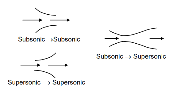.png?revision=1) |
| Physical Features | No work \((\dot{W} = 0)\) One-inlet / one-outlet |
|
| Operating Conditions | Steady-state system One-dimensional flow at inlets/outlets Negligible changes in gravitational potential energy Inlet kinetic energy is negligible Negligible heat transfer for the system (adiabatic system, \(\dot{Q} = 0\)) Best performance: Reversible and adiabatic |
|
(1) Sketch a typical nozzle and label the inlet 1 and the outlet 2 .
(2) Develop a model for this device using the information above to simplify the rate form of the conservation of mass and the conservation of energy equations. \[\begin{aligned} &\frac{d}{dt} \left(m_{sys}\right) = \dot{m}_{1}-\dot{m}_{2} \\ &\frac{d}{dt} \left(E_{sys}\right) = \dot{Q}_{\text{net, in}} + \dot{W}_{\text{net, in}} + \dot{m}_{1} \left(h_{1}+\frac{V_{1}^{2}}{2}+g z_{1}\right) - \dot{m}_{2} \left(h_{2}+\frac{V_{2}^{2}}{2}+g z_{2}\right) \end{aligned} \nonumber \]
| Device Name(s) | Diffusers | |
|---|---|---|
| Purpose | Increase pressure while decreasing flow velocity (kinetic energy) in the direction of flow. | 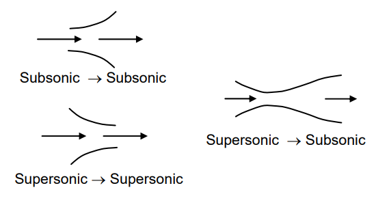.png?revision=1) |
| Physical Features | No work \((\dot{W}=0)\) One-inlet / one-outlet |
|
| Operating Conditions | Steady-state system One-dimensional flow at inlets/outlets Negligible changes in gravitational potential energy Outlet kinetic energy is negligible Negligible heat transfer for the system (adiabatic system, \(\dot{Q} = 0\)) Best performance: Reversible and adiabatic |
|
(1) Sketch a typical diffuser and label the inlet 1 and the outlet 2 .
(2) Develop a model for this device using the information above to simplify the rate form of the conservation of mass and the conservation of energy equations. \[\begin{aligned} &\frac{d}{dt}\left(m_{sys}\right) = \dot{m}_{1}-\dot{m}_{2} \\ &\frac{d}{dt}\left(E_{sys}\right) = \dot{Q}_{\text{net, in}} + \dot{W}_{\text{net, in}} + \dot{m}_{1} \left(h_{1}+\frac{V_{1}^{2}}{2}+g z_{1}\right) - \dot{m}_{2} \left(h_{2}+\frac{V_{2}^{2}}{2}+g z_{2}\right) \end{aligned} \nonumber \]
| Device Name(s) | Throttling Devices | |
|---|---|---|
| Purpose | Decrease pressure in the direction of flow. | .png?revision=1) |
| Physical Features | No work \((\dot{W} = 0)\) One-inlet / one-outlet |
|
| Operating Conditions | Steady-state system One-dimensional flow at inlets/outlets Negligible changes in gravitational potential energy Negligible changes in kinetic energy Negligible heat transfer for the system (adiabatic system, \(\dot{Q} = 0\)) |
|
(1) Sketch a typical throttling valve and label the inlet 1 and the outlet 2.
(2) Develop a model for this device using the information above to simplify the rate form of the conservation of mass and the conservation of energy equations. \[\begin{aligned} &\frac{d}{dt} \left(m_{sys}\right) = \dot{m}_{1}-\dot{m}_{2} \\ &\frac{d}{dt} \left(E_{sys}\right) = \dot{Q}_{\text{net, in}} + \dot{W}_{\text{net, in}} + \dot{m}_{1}\left(h_{1}+\frac{V_{1}^{2}}{2}+g z_{1}\right) - \dot{m}_{2}\left(h_{2}+\frac{V_{2}^{2}}{2}+g z_{2}\right) \end{aligned} \nonumber \]
Turbines and Pumps, Compressors, Blowers, and Fans
Turbines and pumps, compressors, blowers and fans all do the same thing—they alter the properties of a flowing fluid by transferring energy by work into or out of the fluid. The tables below provide additional information about each of these devices. Look for the similarities and the unique differences.
| Device Name(s) | Turbines | |
|---|---|---|
| Purpose | Produce mechanical power (shaft power) from a flowing stream of fluid. | .png?revision=1) |
| Physical Features | Mechanical power output \((\dot{W}_{\text {out }}>0)\) Often one-inlet/one-outlet |
|
| Operating Conditions | Steady-state system One-dimensional flow at inlets/outlets Negligible changes in gravitational potential energy Negligible changes in kinetic energy Negligible heat transfer for the system (adiabatic system, \(\dot{Q} = 0\)) Best performance: Reversible and adiabatic |
|
(1) Sketch a typical turbine and label the inlet 1 and the outlet 2.
(2) Develop a model for this device using the information above to simplify the rate form of the conservation of mass and the conservation of energy equations. \[\begin{aligned} &\frac{d}{dt} \left(m_{sys}\right) = \dot{m}_{1}-\dot{m}_{2} \\ &\frac{d}{dt} \left(E_{sys}\right) = \dot{Q}_{\text {net, in}} + \dot{W}_{\text {net, in}} + \dot{m}_{1} \left(h_{1}+\frac{V_{1}^{2}}{2}+g z_{1}\right) - \dot{m}_{2} \left(h_{2}+\frac{V_{2}^{2}}{2}+g z_{2}\right) \end{aligned} \nonumber \]
| Device Name(s) | Pumps, Compressors, Blowers, and Fans | |
|---|---|---|
| Purpose | Move, compress, and/or increase the pressure of a fluid. | .png?revision=1) |
| Physical Features | Mechanical power input \((\dot{W}_{\text{in}} >0)\) Usually one-inlet / one-outlet Pump \(\rightarrow\) Liquids, large or small \(\Delta \mathrm{P}\) Compressors \(\rightarrow\) gases, large \(\Delta \mathrm{P}\) Blowers \(\rightarrow\) gases, small \(\Delta \mathrm{P}\) Fans \(\rightarrow\) gases, very small \(\Delta \mathrm{P}\) |
|
| Operating Conditions | Steady-state system One-dimensional flow at inlets/outlets Negligible changes in gravitational potential energy Negligible changes in kinetic energy Negligible heat transfer for the system (adiabatic system, \(\dot{Q}=0\)) Best performance: Reversible and adiabatic |
|
(1) Sketch a typical compressor and label the inlet 1 and the outlet 2.
(2) Develop a model for this device using the information above to simplify the rate form of the conservation of mass and the conservation of energy equations. \[\begin{aligned} &\frac{d}{dt} \left(m_{sys}\right) = \dot{m}_{1}-\dot{m}_{2} \\ &\frac{d}{dt} \left(E_{sys}\right) = \dot{Q}_{\text{net, in}} + \dot{W}_{\text{net, in}} + \dot{m}_{1}\left(h_{1}+\frac{V_{1}^{2}}{2}+g z_{1}\right) - \dot{m}_{2}\left(h_{2}+\frac{V_{2}^{2}}{2}+g z_{2}\right) \end{aligned} \nonumber \]
Heat Exchangers
Heat exchangers are devices designed to change the property of a flowing fluid by transferring energy by heat transfer into or out of a system. Some designs keep the fluids separate, such as in the radiator of your car. These are heat exchangers without mixing. Other times the fluids are typically mixed, such as in the plumbing to your shower—you adjust the temperature of the water by changing the flow rates of the hot and cold water. This is known as a heat exchanger with mixing. The tables below provide additional information about each of these devices. Look for the similarities and the unique differences.
| Device Name(s) | Heat Exchangers without Mixing | |
|---|---|---|
| Purpose | Transfer thermal energy between fluid streams. | .png?revision=1) |
| Physical Features | No work \((\dot{W}=0)\) Separate flow paths for each stream (no mixing). |
|
| Operating Conditions | Steady-state system One-dimensional flow at inlets/outlets Negligible changes in gravitational potential energy Negligible changes in kinetic energy Negligible pressure drop for each stream (isobaric) Negligible heat transfer for the overall system (adiabatic system, \(\dot{Q} = 0\)) (This is not true if either fluid stream alone is the system.) |
|
(1) Sketch a typical heat exchanger without mixing with two fluid streams — a hot stream and a cold stream. Label the inlet and the outlet of the cold stream \(\mathrm{C}1\) and \(\mathrm{C}2\). Label the inlet and the outlet of the hot stream \(\mathrm{H}1\) and \(\mathrm{H}2\).
(2) Develop a model for this device using the information above to simplify the rate form of the conservation of mass and the conservation of energy equations.
System is the Hot Stream
\[\begin{aligned} & \frac{d}{dt}\left(m_{sys}\right) = \dot{m}_{H1}-\dot{m}_{H2} \\ & \frac{d}{dt} \left(E_{sys}\right) = \dot{Q}_{\text{net, in}} + \dot{W}_{\text{net, in}} + \dot{m}_{H1} \left(h_{H1}+\frac{V_{H1}{ }^{2}}{2}+g z_{H1}\right) - \dot{m}_{H2} \left(h_{H2}+\frac{V_{H2}{ }^{2}}{2}+g z_{H2}\right) \end{aligned} \nonumber \]
System is the Cold Stream
\[\begin{aligned} &\frac{d}{dt}\left(m_{sys}\right) = \dot{m}_{C1}-\dot{m}_{C2} \\ &\frac{d}{dt}\left(E_{sys}\right) = \dot{Q}_{\text{net, in}} + \dot{W}_{\text{net, in}} +\dot{m}_{C1} \left(h_{C1}+\frac{V_{C1}{ }^{2}}{2}+g z_{C 1}\right) - \dot{m}_{C2} \left(h_{C2}+\frac{V_{C2}{ }^{2}}{2}+g z_{C2}\right) \end{aligned} \nonumber \]
System is the Complete Heat Exchanger
\[\begin{aligned} &\frac{d}{dt}\left(m_{sys}\right) = \dot{m}_{C1}-\dot{m}_{C2}+\dot{m}_{H1}-\dot{m}_{H2} \\ & \frac{d}{dt} \left(E_{sys}\right) = \dot{Q}_{\text{net, in}} + \dot{W}_{\text{net, in}} + \dot{m}_{C1} \left(h_{C1}+\frac{V_{C1}{ }^{2}}{2}+g z_{C1}\right) - \dot{m}_{C2} \left(h_{C2}+\frac{V_{C2}{ }^{2}}{2}+g z_{C2}\right) + \\ &\quad\quad\quad\quad\quad\quad \dot{m}_{H1}\left(h_{H1}+\frac{V_{H1}{ }^{2}}{2}+g z_{H1}\right) - \dot{m}_{H2} \left(h_{H2}+\frac{V_{H2}{ }^{2}}{2}+g z_{H2}\right) \end{aligned} \nonumber \]
| Device Name(s) | Heat Exchangers with Mixing | |
|---|---|---|
| Purpose | Transfer thermal energy between fluid streams. | .png?revision=1) |
| Physical Features | Fluid streams mix No work \((\dot{W}=0)\) |
|
| Operating Conditions | Steady-state system One-dimensional flow at inlets/outlets Negligible changes in gravitational potential energy Negligible changes in kinetic energy Negligible pressure drop (isobaric) Negligible heat transfer for the overall system (adiabatic system, \(\dot{Q}=0)\) |
|
(1) Sketch a typical heat exchanger with mixing with two fluid streams — a hot stream and a cold stream. Label the two inlet streams \(1\) and \(2\) and the outlet stream \(3\).
(2) Develop a model for this device using the information above to simplify the rate form of the conservation of mass and the conservation of energy equations.
\[\begin{aligned} &\frac{d}{dt}\left(m_{sys}\right) = \dot{m}_{1}+\dot{m}_{2}-\dot{m}_{3} \\ &\frac{d}{dt}\left(E_{sys}\right) = \dot{Q}_{\text{net, in}} + \dot{W}_{\text {net, in}} + \dot{m}_{1} \left(h_{1}+\frac{V_{1}^{2}}{2}+g z_{1}\right) + \dot{m}_{2} \left(h_{2}+\frac{V_{2}^{2}}{2}+g z_{2}\right) - \dot{m}_{3}\left(h_{3}+\frac{V_{3}^{2}}{2}+g z_{3}\right) \end{aligned} \nonumber \]