10: Parachute Person
- Page ID
- 40964
\( \newcommand{\vecs}[1]{\overset { \scriptstyle \rightharpoonup} {\mathbf{#1}} } \)
\( \newcommand{\vecd}[1]{\overset{-\!-\!\rightharpoonup}{\vphantom{a}\smash {#1}}} \)
\( \newcommand{\dsum}{\displaystyle\sum\limits} \)
\( \newcommand{\dint}{\displaystyle\int\limits} \)
\( \newcommand{\dlim}{\displaystyle\lim\limits} \)
\( \newcommand{\id}{\mathrm{id}}\) \( \newcommand{\Span}{\mathrm{span}}\)
( \newcommand{\kernel}{\mathrm{null}\,}\) \( \newcommand{\range}{\mathrm{range}\,}\)
\( \newcommand{\RealPart}{\mathrm{Re}}\) \( \newcommand{\ImaginaryPart}{\mathrm{Im}}\)
\( \newcommand{\Argument}{\mathrm{Arg}}\) \( \newcommand{\norm}[1]{\| #1 \|}\)
\( \newcommand{\inner}[2]{\langle #1, #2 \rangle}\)
\( \newcommand{\Span}{\mathrm{span}}\)
\( \newcommand{\id}{\mathrm{id}}\)
\( \newcommand{\Span}{\mathrm{span}}\)
\( \newcommand{\kernel}{\mathrm{null}\,}\)
\( \newcommand{\range}{\mathrm{range}\,}\)
\( \newcommand{\RealPart}{\mathrm{Re}}\)
\( \newcommand{\ImaginaryPart}{\mathrm{Im}}\)
\( \newcommand{\Argument}{\mathrm{Arg}}\)
\( \newcommand{\norm}[1]{\| #1 \|}\)
\( \newcommand{\inner}[2]{\langle #1, #2 \rangle}\)
\( \newcommand{\Span}{\mathrm{span}}\) \( \newcommand{\AA}{\unicode[.8,0]{x212B}}\)
\( \newcommand{\vectorA}[1]{\vec{#1}} % arrow\)
\( \newcommand{\vectorAt}[1]{\vec{\text{#1}}} % arrow\)
\( \newcommand{\vectorB}[1]{\overset { \scriptstyle \rightharpoonup} {\mathbf{#1}} } \)
\( \newcommand{\vectorC}[1]{\textbf{#1}} \)
\( \newcommand{\vectorD}[1]{\overrightarrow{#1}} \)
\( \newcommand{\vectorDt}[1]{\overrightarrow{\text{#1}}} \)
\( \newcommand{\vectE}[1]{\overset{-\!-\!\rightharpoonup}{\vphantom{a}\smash{\mathbf {#1}}}} \)
\( \newcommand{\vecs}[1]{\overset { \scriptstyle \rightharpoonup} {\mathbf{#1}} } \)
\(\newcommand{\longvect}{\overrightarrow}\)
\( \newcommand{\vecd}[1]{\overset{-\!-\!\rightharpoonup}{\vphantom{a}\smash {#1}}} \)
\(\newcommand{\avec}{\mathbf a}\) \(\newcommand{\bvec}{\mathbf b}\) \(\newcommand{\cvec}{\mathbf c}\) \(\newcommand{\dvec}{\mathbf d}\) \(\newcommand{\dtil}{\widetilde{\mathbf d}}\) \(\newcommand{\evec}{\mathbf e}\) \(\newcommand{\fvec}{\mathbf f}\) \(\newcommand{\nvec}{\mathbf n}\) \(\newcommand{\pvec}{\mathbf p}\) \(\newcommand{\qvec}{\mathbf q}\) \(\newcommand{\svec}{\mathbf s}\) \(\newcommand{\tvec}{\mathbf t}\) \(\newcommand{\uvec}{\mathbf u}\) \(\newcommand{\vvec}{\mathbf v}\) \(\newcommand{\wvec}{\mathbf w}\) \(\newcommand{\xvec}{\mathbf x}\) \(\newcommand{\yvec}{\mathbf y}\) \(\newcommand{\zvec}{\mathbf z}\) \(\newcommand{\rvec}{\mathbf r}\) \(\newcommand{\mvec}{\mathbf m}\) \(\newcommand{\zerovec}{\mathbf 0}\) \(\newcommand{\onevec}{\mathbf 1}\) \(\newcommand{\real}{\mathbb R}\) \(\newcommand{\twovec}[2]{\left[\begin{array}{r}#1 \\ #2 \end{array}\right]}\) \(\newcommand{\ctwovec}[2]{\left[\begin{array}{c}#1 \\ #2 \end{array}\right]}\) \(\newcommand{\threevec}[3]{\left[\begin{array}{r}#1 \\ #2 \\ #3 \end{array}\right]}\) \(\newcommand{\cthreevec}[3]{\left[\begin{array}{c}#1 \\ #2 \\ #3 \end{array}\right]}\) \(\newcommand{\fourvec}[4]{\left[\begin{array}{r}#1 \\ #2 \\ #3 \\ #4 \end{array}\right]}\) \(\newcommand{\cfourvec}[4]{\left[\begin{array}{c}#1 \\ #2 \\ #3 \\ #4 \end{array}\right]}\) \(\newcommand{\fivevec}[5]{\left[\begin{array}{r}#1 \\ #2 \\ #3 \\ #4 \\ #5 \\ \end{array}\right]}\) \(\newcommand{\cfivevec}[5]{\left[\begin{array}{c}#1 \\ #2 \\ #3 \\ #4 \\ #5 \\ \end{array}\right]}\) \(\newcommand{\mattwo}[4]{\left[\begin{array}{rr}#1 \amp #2 \\ #3 \amp #4 \\ \end{array}\right]}\) \(\newcommand{\laspan}[1]{\text{Span}\{#1\}}\) \(\newcommand{\bcal}{\cal B}\) \(\newcommand{\ccal}{\cal C}\) \(\newcommand{\scal}{\cal S}\) \(\newcommand{\wcal}{\cal W}\) \(\newcommand{\ecal}{\cal E}\) \(\newcommand{\coords}[2]{\left\{#1\right\}_{#2}}\) \(\newcommand{\gray}[1]{\color{gray}{#1}}\) \(\newcommand{\lgray}[1]{\color{lightgray}{#1}}\) \(\newcommand{\rank}{\operatorname{rank}}\) \(\newcommand{\row}{\text{Row}}\) \(\newcommand{\col}{\text{Col}}\) \(\renewcommand{\row}{\text{Row}}\) \(\newcommand{\nul}{\text{Nul}}\) \(\newcommand{\var}{\text{Var}}\) \(\newcommand{\corr}{\text{corr}}\) \(\newcommand{\len}[1]{\left|#1\right|}\) \(\newcommand{\bbar}{\overline{\bvec}}\) \(\newcommand{\bhat}{\widehat{\bvec}}\) \(\newcommand{\bperp}{\bvec^\perp}\) \(\newcommand{\xhat}{\widehat{\xvec}}\) \(\newcommand{\vhat}{\widehat{\vvec}}\) \(\newcommand{\uhat}{\widehat{\uvec}}\) \(\newcommand{\what}{\widehat{\wvec}}\) \(\newcommand{\Sighat}{\widehat{\Sigma}}\) \(\newcommand{\lt}{<}\) \(\newcommand{\gt}{>}\) \(\newcommand{\amp}{&}\) \(\definecolor{fillinmathshade}{gray}{0.9}\)Parachute person is an example of a problem relevant to engineers and scientists that can be made fairly simple for beginning programmers. This problem can be analytically solved using differential equations, however, there are many problems that cannot be solved analytically, but can be solved on a computer using an approximation method (a simple numerical method which in this case makes an approximation of a differential equation).
So why write a program if it can be solved analytically? Because this program is simpler than an intractable problem (that you would more likely write a program for) and thus will be easier to grasp for a beginning programmer. Will real world problems be as simple? No. This example can be expanded to intractable real world problems, but a good understanding of numerical methods is necessary to truly do this sort of work (therefore it is wise for a student to take a numerical methods course or a signals and systems course that includes numerical methods).
First we discuss the physics and show how to design a computer program from a "word" problem. Then we show the working program and the results we can get.
So lets start with the problem.
A person has jumped out of a plane with a parachute, what is the velocity as the person reaches the ground?
As with all programming an initial program is made and then new versions enhance the initial program. Assumptions can systematically be removed or refined for new versions, but for now we will do the initial program. Because this is such a general problem the instructor has obviously :) given us liberty to make some reasonable assumptions. So let us list some assumptions.
- The ground is sufficiently far enough that the parachutist doesn't hit the ground before reaching terminal velocity
- The parachutist opens the parachute as soon as he jumps out of the plane (this of course would be one of the first assumptions to be revisited)
- The drag constant will include drag coefficient, parachute area size, design of parachute, and density of the air (more assumptions that would eventually be revisited)
- Weight of parachute is negligible
- Wind will be assumed to be zero in all directions (this assumption might be difficult to revisit, but give it a shot when you are more expert at programming)
So this is a physics problem at its heart. Since the parachutist is moving we recognize this as a dynamic problem.
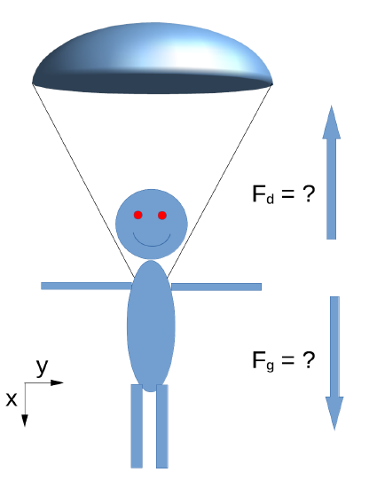
- First step in a dynamic physics problem is to set up your force diagram.
- Before you draw your force diagram, draw your coordinate directions (which way does "x" go....which way does "y" go)
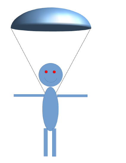
- Use the parachutist below to draw your forces.

- ¬ Parachute dude's force diagram (with coordinate system)
-

Good, so we now see that the drag force (\(F_d\)) is negative (because of the coordinate system) and the gravity force (\(F_g\)) is positive. Now what do the forces equal? Assume a generic constant for the drag force.
- ¬ Forces defined
-
\[{\vec{F_g}} = \frac{d{\vec{p}}} {dt}\]
Assuming m is constant we can rewrite this as...
\[{\vec{F_g}} = m \vec{a} = mg\]
The simplest version of the drag force is this...
\[{\vec{F_d}} = c v^2\]
Where c represents a constant that incorporates the drag coefficient, cross sectional area of the parachute, and the density of the atmosphere...
- ¬ Force equation
-
The generic static rule is that the sum of the forces in one direction equal zero (in addition to other equations introduced later)
\[\sum{F_i} = 0\]
However this problem is not static, it is dynamic, so...
\[\sum{F_i} = ma \]
Given our previously defined forces with their directions we have as a final equation
\[F_g - F_d = mg - c v^2 = ma\]
Using a differential for the acceleration we will develop a simple differential equation
\[mg - c v^2 = m \frac{dv}{dt}\]
While we could solve this differential equation using standard ideas introduced in differential equations (which most of you haven't taken), that is not the point of this exercise (whew!), so the next step is to produce an equation suitable for incorporating into a computer program.
- ¬ Force equation redefined...this is where it moves from physics to computer science
-
Starting with the differential equation previously derived
\[ m \frac{dv}{dt} = mg - c v^2\]
and the definition of a differential
\[ \frac{dv}{dt} = \lim_{t \to 0} \frac{\Delta v}{\Delta t}\]
we can write an approximate "algebraic" equation
\[ \frac{\Delta v}{\Delta t} = g - \frac{c}{m} v^2\]
which we will rewrite as
\[ {\Delta v} = (g - \frac{c}{m} v^2) {\Delta t} \]
This is the form we will make into a usable computer form by using the definition of what the delta means in mathematics...which is
\[ {\Delta v} = v_{i+1} - v_{i} \]
Substituting into the previous equation we have
\[ v_{i+1} - v_{i} = (g - \frac{c}{m} (v_{i})^2) {\Delta t} \]
Which we then rewrite in a form that is recognized as Euler's method in numerical methods...
\[ v_{i+1} = v_{i} + (g - \frac{c}{m} (v_{i})^2) {\Delta t} \]
A vector (array) form is useful when writing a computer program as subscripts are not recognized by computer languages
\[ v(i+1) = v(i) + (g - c*(v(i))^2/m) * tsteps \]
Now we are ready to program this...yes!!!
- ¬ Vector array, say what?
-
The vector array as noted previously is a variable that has many cells. Below is an example where t and v are vector arrays. This means that t and v are actually many variables as one. If we define v (in Fortran, say) as -- double, dimension(10) :: v -- then v is actually 10 distinct variables having the names v(1), v(2), v(3), v(4), v(5), v(6), v(7), v(8), v(9), and v(10). Each of these variables can be assigned a number as the example below shows.
i is an index variable t(i) is time (seconds) v(i) is velocity 1 0.0 0.0 2 0.1 0.98 3 0.2 1.93253 4 0.3 2.80572 5 0.4 3.56058 6 0.5 4.17800 7 0.6 4.65876 8 0.7 5.01803 ... ... ... -
The previous example fits with the final program below...
Parachute person as presented here becomes more complex as we remove the simplified assumptions. Final solutions (as in the program, not the "answer") would involve fluid dynamics and would likely be a system of equations (usually expressed in matrix form).

