Chapter 14: Composites

Composite Mechanics:

So far we have been talking about the mechanics of primarily polymers but we haven’t really touched on composite mechanics. Composites materials are materials that contain typically more than one type of material combined. This typically involves a material matrix which is the major component in terms of volume fraction. This matrix material is reinforced by an additional material typically one that is stiffer or tougher than matrix material. The material that reinforces the matrix can be in particle form, fibers, or precipitates. A composite can also be a porous material like metal foams, concrete, ECM, etc.

Let’s take a look at a particle reinforced composite that is composed of a matrix which has some elastic modulus, E_m, and volume fraction, f_m. There is also the particle reinforcement in this case which again has an associated elastic modulus, E_p, and volume fraction f_p. Thus the total composite modulus, E_composite is

$$E_{composite} = E_{m}f_{m} + E_{p}f_{p} \nonumber$$

empirically there is typically a constant that is less than 1 for the particle reinforcement contribution but again that constant can only be found empirically.

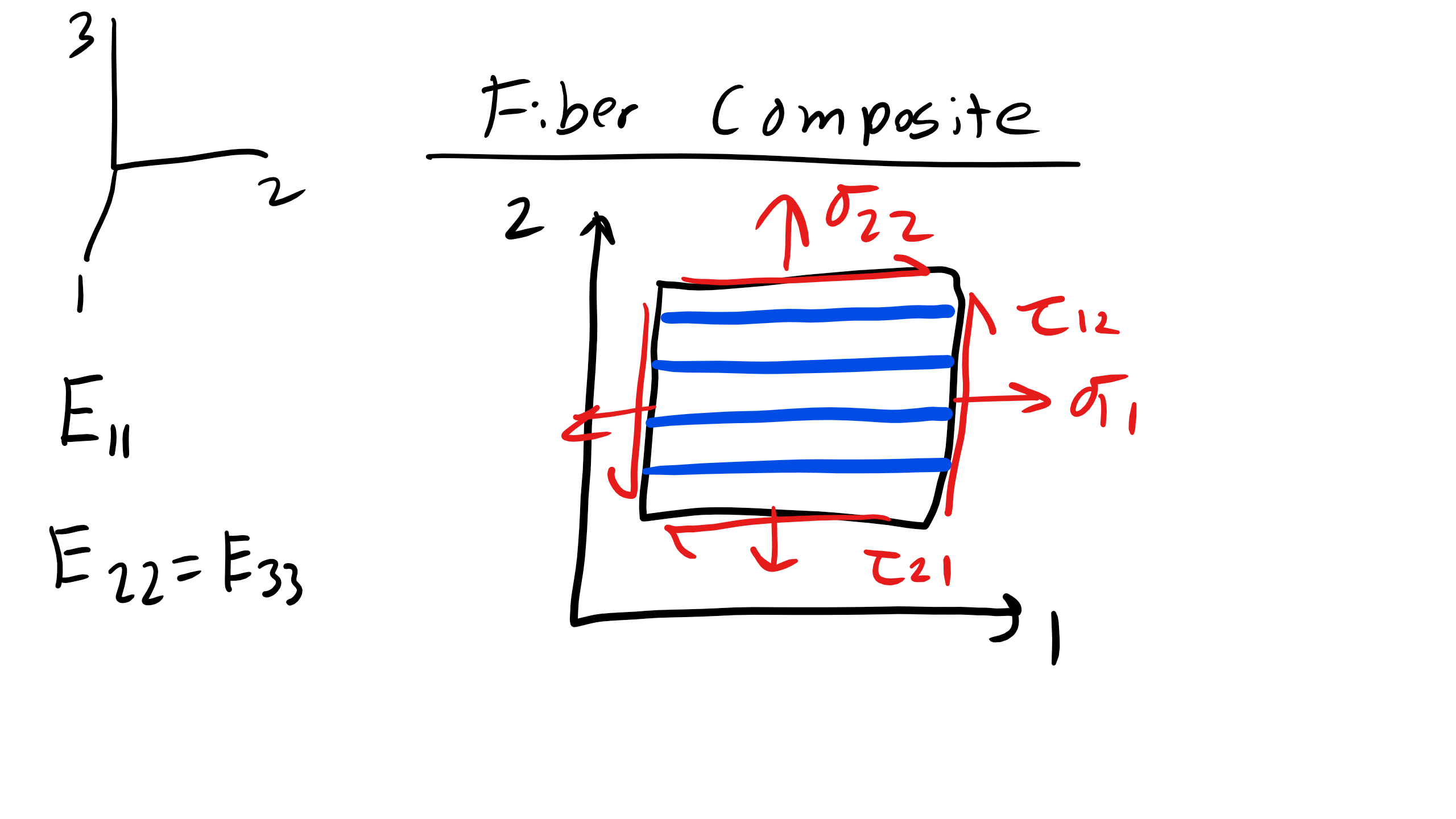
Let’s now look at a fiber reinforced composite that is pulled or stressed in the transverse direction with respect the the longitudinal or axial direction of the fibers. The stresses are the same on the matrix and the fibers. However the strains of the fiber and matrix will be different. With these constraints:

$$\sigma_{m} = \sigma_{f} = \sigma \nonumber$$

$$\epsilon_{c} = \epsilon_{m}f_{m} + \epsilon_{f}f_{f} \nonumber$$

$$\epsilon_{c} = \sigma \bigg(\frac{f_{m}}{E_{m}} + \frac{f_{f}}{E_{f}}\bigg) \nonumber$$

$$\frac{1}{E_{c}} = \frac{f_{f}}{E_{f}} + \frac{f_{m}}{E_{m}} \nonumber$$

If we instead pull parallel to the fiber longitudinal or axial direction. Here the strain is the same but now the stresses will be different for the fibers and the matrix. So with those constraints we get

$$\sigma_{c} = \sigma_{f}f_{f} + \sigma_{m}f_{m} \nonumber$$

$$\epsilon_{c} = \epsilon_{m} = \epsilon_{f} \nonumber$$

$$\sigma_{c} = E_{f}\epsilon f_{f} + E_{m}\epsilon f_{m} \nonumber$$

$$E_{c} = E_{f}f_{f} + E_{m}f_{m} \nonumber$$

We can see the difference in the Young’s modulus in both of these directions as function of volume fraction in the plot below:

Transversely Isotropic Composite

Let’s go a bit further and do an example of a composite or laminate that is transversely isotropic (i.e. E₃₃ = E₂₂ 6= E₁₁).

In this scenario our compliance and stiffness matrices would like like this

$$\begin{bmatrix} \sigma_1\\ \sigma_2\\ \sigma_3\\ \sigma_4\\ \sigma_5\\ \sigma_6 \end{bmatrix} = \begin{bmatrix} C_{11} & C_{12} & C_{13} & 0 & 0 & 0 \\ C_{12} & C_{22} & C_{13} & 0 & 0 & 0 \\ C_{13} & C_{13} & C_{33} & 0 & 0 & 0 \\ 0 & 0 & 0 & C_{44} & 0 & 0 \\ 0 & 0 & 0 & 0 & C_{44} & 0 \\ 0 & 0 & 0 & 0 & 0 & \frac{C_{11} - C_{12}}{2} \\ \end{bmatrix} \begin{bmatrix} \epsilon_1\\ \epsilon_2\\ \epsilon_3\\ \epsilon_4\\ \epsilon_5\\ \epsilon_6 \end{bmatrix} \nonumber$$

or equivalently

$$\begin{bmatrix} \epsilon_1\\ \epsilon_2\\ \epsilon_3\\ \epsilon_4\\ \epsilon_5\\ \epsilon_6 \end{bmatrix} = \begin{bmatrix} \frac{1}{E_{1}} & -\frac{\nu_{21}}{E_{2}} & -\frac{\nu_{31}}{E_{2}} & 0 & 0 & 0 \\ -\frac{\nu_{12}}{E_{1}} & \frac{1}{E_{2}} & -\frac{\nu_{32}}{E_{2}} & 0 & 0 & 0 \\ -\frac{\nu_{13}}{E_{1}} & -\frac{\nu_{23}}{E_{2}} & \frac{1}{E_{2}} & 0 & 0 & 0 \\ 0 & 0 & 0 & \frac{1}{G_{12}} & 0 & 0 \\ 0 & 0 & 0 & 0 & \frac{1}{G_{23}} & 0 \\ 0 & 0 & 0 & 0 & 0 & \frac{1}{G_{13}} \\ \end{bmatrix} \begin{bmatrix} \sigma_1\\ \sigma_2\\ \sigma_3\\ \sigma_4\\ \sigma_5\\ \sigma_6 \end{bmatrix} \nonumber$$

 

We can see from this that as a result we will have that $\epsilon_4 = \epsilon_5 = 0$. We also know that from our conditions of tensor symmetry that

$$\frac{\nu_{21}}{E_{2}} = \frac{\nu_{12}}{E_{1}} \nonumber$$
$$\frac{\nu_{13}}{E_{1}} = \frac{\nu_{31}}{E_2} \nonumber$$
$$\frac{\nu_{23}}{E_{2}} = \frac{\nu_{32}}{E_2} \nonumber$$

Now a typical scenario for composites will be when they are placed under plane stress conditions and we can then simplify our matrix and only focus on the in-plane stress and strains where we now have

$$\begin{bmatrix} \epsilon_1 \\ \epsilon_2 \\ 0 \\ 0 \\ 0 \\ \epsilon_6 \end{bmatrix} = \begin{bmatrix} \frac{1}{E_{1}} & -\frac{\nu_{21}}{E_{2}} & -\frac{\nu_{31}}{E_2} & 0 & 0 & 0 \\ -\frac{\nu_{12}}{E_{1}} & \frac{1}{E_{2}} & -\frac{\nu_{32}}{E_2} & 0 & 0 & 0 \\ -\frac{\nu_{13}}{E_{1}} & -\frac{\nu_{23}}{E_{2}} & \frac{1}{E_{2}} & 0 & 0 & 0 \\ 0 & 0 & 0 & \frac{1}{G_{12}} & 0 & 0 \\ 0 & 0 & 0 & 0 & \frac{1}{G_{23}} & 0 \\ 0 & 0 & 0 & 0 & 0 & \frac{1}{G_{13}} \\ \end{bmatrix} \begin{bmatrix} \sigma_1 \\ \sigma_2 \\ \sigma_3 \\ \sigma_4 \\ \sigma_5 \\ \sigma_6 \end{bmatrix} \nonumber$$

or more visually appealing

$$\begin{bmatrix} \epsilon_{11} \\ \epsilon_{22} \\ \epsilon_{12} \end{bmatrix} = \begin{bmatrix} \frac{1}{E_{1}} & \frac{-\nu_{21}}{E_{2}} & 0 \\ \frac{-\nu_{12}}{E_{1}} & \frac{1}{E_{2}} & 0 \\ 0 & 0 & \frac{1}{G_{12}} \\ \end{bmatrix} \begin{bmatrix} \sigma_1 \\ \sigma_2 \\ \sigma_{12} \end{bmatrix} \nonumber$$

This great but this is only applies if we are pulling along the principal axes. How can we express the properties of this material when stressed along arbitrary directions with regards to the principal axes. Well we will use linear algebra!

We have previously seen in the elasticity lecture how to rotate stresses and strains in relation to Mohr’s circle and we can do the same thing here. We will use our same rotation matrices, transformation matrix (T), as previously defined and we can obtain stress after an arbitrary rotation

$$\begin{bmatrix} \sigma_{x^{'}} \\ \sigma_{y^{'}} \\ \sigma_{xy^{'}} \end{bmatrix} = \begin{bmatrix} T \end{bmatrix} \begin{bmatrix} \sigma_x \\ \sigma_y \\ \sigma_{xy} \end{bmatrix} \nonumber$$

For strain again we have to deal with this factor of 2 in relating shear strain so first we have to account for $\epsilon_{12} = \frac{\gamma_{12}}{2}$ so we have to introduce another matrix, the Reuter Matrix (R) as previously defined. So to convert to

$$\begin{bmatrix} \epsilon_{x^{'}} \\ \epsilon_{y^{'}} \\ \gamma_{xy^{'}} \end{bmatrix} = RTR^{-1} \begin{bmatrix} \epsilon_x \\ \epsilon_y \\ \gamma_{xy} \end{bmatrix} \nonumber$$

Now we can finally determine the strain at an arbitrary rotation for a transverse isotropic polymer composite or laminate which can be seen below when we combine these expressions

$$\begin{bmatrix} \epsilon_{x^{'}} \\ \epsilon_{y^{'}} \\ \gamma_{xy^{'}} \end{bmatrix} = RTR^{-1}ST^{-1} \begin{bmatrix} \sigma_{x^{'}} \\ \sigma_{y^{'}} \\ \sigma_{xy^{'}} \end{bmatrix} \nonumber$$

Case Study: Block Copolymers Composite Mechanics

In BCPs, we saw a variety of different morphologies based on the phase fraction and temperature of the system. In principal, the anisotropy of these systems gives rise to anisotropy in the mechanical properties as well, since pulling along the axis of a cylinder, for example, will yield a different modulus than pulling perpendicular to the axis.

Let’s consider an example of triblock copolymers forming lamellae, with glassy domains forming one lamella and rubbery domains forming the other. This would occur if two of the blocks in the triblock have very different glass transition temperatures, such that one would be glassy while the other rubbery. We can now treat the mechanical properties in much the same way as we would treat composities . Pulling along the axis of the lamellae (that is, along the long edge) leads to pulling on actual glassy domains, since in order to deform in this direction both rubbery and glassy lamellae have to elongate by an equal amount. Since the modulus of the glassy domain is much higher, the glassy modulus will essentially be the only contributor to the measured modulus in this direction.

If you pull at 90^o to the axis (i.e. in the direction that intersects each face of the lamellae), then the rubbery regions will preferentially deform first since their modulus is much lower, and the glassy domains will not deform at all. The modulus in this direction is dominated by the rubbery modulus, though higher because of the constraints of maintaining a lamellar geometry.

The surprising result, though, is that when pulling at 45^o, the modulus is lowest - this is because the material is being sheared at constant volume. At 90^o, the uniaxial deformation leads to necking which attempts to change the volume of the sample locally - think of the rubbery polymers stretching out and thinning the sample while still aggregating laterally, which leads to bowing. Pulling at 45^o, however, applies stress along the axis of maximum shear stress, leading to shear at constant volume and minimizing the modulus felt.

In the limit of high strains, all of the moduli tend to converge together. The explanation behind this behavior is the onset of kinks - independent of what direction you are applying the stress, eventually the material will reorient to a lowest-energy configuration, which can result in lamellae ”kinking” such that they are at 45^o to the pulling direction, which as noted above has the lowest modulus (and hence lowest energy for a given strain). Some strain energy is thus localized to each kinking point, but overall the morphology can sustain much greater energy by putting energy into shearing the lamellae at 45^o, the preferred direction.