5: Molecular Weight Averages
- Page ID
- 2908
\( \newcommand{\vecs}[1]{\overset { \scriptstyle \rightharpoonup} {\mathbf{#1}} } \)
\( \newcommand{\vecd}[1]{\overset{-\!-\!\rightharpoonup}{\vphantom{a}\smash {#1}}} \)
\( \newcommand{\dsum}{\displaystyle\sum\limits} \)
\( \newcommand{\dint}{\displaystyle\int\limits} \)
\( \newcommand{\dlim}{\displaystyle\lim\limits} \)
\( \newcommand{\id}{\mathrm{id}}\) \( \newcommand{\Span}{\mathrm{span}}\)
( \newcommand{\kernel}{\mathrm{null}\,}\) \( \newcommand{\range}{\mathrm{range}\,}\)
\( \newcommand{\RealPart}{\mathrm{Re}}\) \( \newcommand{\ImaginaryPart}{\mathrm{Im}}\)
\( \newcommand{\Argument}{\mathrm{Arg}}\) \( \newcommand{\norm}[1]{\| #1 \|}\)
\( \newcommand{\inner}[2]{\langle #1, #2 \rangle}\)
\( \newcommand{\Span}{\mathrm{span}}\)
\( \newcommand{\id}{\mathrm{id}}\)
\( \newcommand{\Span}{\mathrm{span}}\)
\( \newcommand{\kernel}{\mathrm{null}\,}\)
\( \newcommand{\range}{\mathrm{range}\,}\)
\( \newcommand{\RealPart}{\mathrm{Re}}\)
\( \newcommand{\ImaginaryPart}{\mathrm{Im}}\)
\( \newcommand{\Argument}{\mathrm{Arg}}\)
\( \newcommand{\norm}[1]{\| #1 \|}\)
\( \newcommand{\inner}[2]{\langle #1, #2 \rangle}\)
\( \newcommand{\Span}{\mathrm{span}}\) \( \newcommand{\AA}{\unicode[.8,0]{x212B}}\)
\( \newcommand{\vectorA}[1]{\vec{#1}} % arrow\)
\( \newcommand{\vectorAt}[1]{\vec{\text{#1}}} % arrow\)
\( \newcommand{\vectorB}[1]{\overset { \scriptstyle \rightharpoonup} {\mathbf{#1}} } \)
\( \newcommand{\vectorC}[1]{\textbf{#1}} \)
\( \newcommand{\vectorD}[1]{\overrightarrow{#1}} \)
\( \newcommand{\vectorDt}[1]{\overrightarrow{\text{#1}}} \)
\( \newcommand{\vectE}[1]{\overset{-\!-\!\rightharpoonup}{\vphantom{a}\smash{\mathbf {#1}}}} \)
\( \newcommand{\vecs}[1]{\overset { \scriptstyle \rightharpoonup} {\mathbf{#1}} } \)
\(\newcommand{\longvect}{\overrightarrow}\)
\( \newcommand{\vecd}[1]{\overset{-\!-\!\rightharpoonup}{\vphantom{a}\smash {#1}}} \)
\(\newcommand{\avec}{\mathbf a}\) \(\newcommand{\bvec}{\mathbf b}\) \(\newcommand{\cvec}{\mathbf c}\) \(\newcommand{\dvec}{\mathbf d}\) \(\newcommand{\dtil}{\widetilde{\mathbf d}}\) \(\newcommand{\evec}{\mathbf e}\) \(\newcommand{\fvec}{\mathbf f}\) \(\newcommand{\nvec}{\mathbf n}\) \(\newcommand{\pvec}{\mathbf p}\) \(\newcommand{\qvec}{\mathbf q}\) \(\newcommand{\svec}{\mathbf s}\) \(\newcommand{\tvec}{\mathbf t}\) \(\newcommand{\uvec}{\mathbf u}\) \(\newcommand{\vvec}{\mathbf v}\) \(\newcommand{\wvec}{\mathbf w}\) \(\newcommand{\xvec}{\mathbf x}\) \(\newcommand{\yvec}{\mathbf y}\) \(\newcommand{\zvec}{\mathbf z}\) \(\newcommand{\rvec}{\mathbf r}\) \(\newcommand{\mvec}{\mathbf m}\) \(\newcommand{\zerovec}{\mathbf 0}\) \(\newcommand{\onevec}{\mathbf 1}\) \(\newcommand{\real}{\mathbb R}\) \(\newcommand{\twovec}[2]{\left[\begin{array}{r}#1 \\ #2 \end{array}\right]}\) \(\newcommand{\ctwovec}[2]{\left[\begin{array}{c}#1 \\ #2 \end{array}\right]}\) \(\newcommand{\threevec}[3]{\left[\begin{array}{r}#1 \\ #2 \\ #3 \end{array}\right]}\) \(\newcommand{\cthreevec}[3]{\left[\begin{array}{c}#1 \\ #2 \\ #3 \end{array}\right]}\) \(\newcommand{\fourvec}[4]{\left[\begin{array}{r}#1 \\ #2 \\ #3 \\ #4 \end{array}\right]}\) \(\newcommand{\cfourvec}[4]{\left[\begin{array}{c}#1 \\ #2 \\ #3 \\ #4 \end{array}\right]}\) \(\newcommand{\fivevec}[5]{\left[\begin{array}{r}#1 \\ #2 \\ #3 \\ #4 \\ #5 \\ \end{array}\right]}\) \(\newcommand{\cfivevec}[5]{\left[\begin{array}{c}#1 \\ #2 \\ #3 \\ #4 \\ #5 \\ \end{array}\right]}\) \(\newcommand{\mattwo}[4]{\left[\begin{array}{rr}#1 \amp #2 \\ #3 \amp #4 \\ \end{array}\right]}\) \(\newcommand{\laspan}[1]{\text{Span}\{#1\}}\) \(\newcommand{\bcal}{\cal B}\) \(\newcommand{\ccal}{\cal C}\) \(\newcommand{\scal}{\cal S}\) \(\newcommand{\wcal}{\cal W}\) \(\newcommand{\ecal}{\cal E}\) \(\newcommand{\coords}[2]{\left\{#1\right\}_{#2}}\) \(\newcommand{\gray}[1]{\color{gray}{#1}}\) \(\newcommand{\lgray}[1]{\color{lightgray}{#1}}\) \(\newcommand{\rank}{\operatorname{rank}}\) \(\newcommand{\row}{\text{Row}}\) \(\newcommand{\col}{\text{Col}}\) \(\renewcommand{\row}{\text{Row}}\) \(\newcommand{\nul}{\text{Nul}}\) \(\newcommand{\var}{\text{Var}}\) \(\newcommand{\corr}{\text{corr}}\) \(\newcommand{\len}[1]{\left|#1\right|}\) \(\newcommand{\bbar}{\overline{\bvec}}\) \(\newcommand{\bhat}{\widehat{\bvec}}\) \(\newcommand{\bperp}{\bvec^\perp}\) \(\newcommand{\xhat}{\widehat{\xvec}}\) \(\newcommand{\vhat}{\widehat{\vvec}}\) \(\newcommand{\uhat}{\widehat{\uvec}}\) \(\newcommand{\what}{\widehat{\wvec}}\) \(\newcommand{\Sighat}{\widehat{\Sigma}}\) \(\newcommand{\lt}{<}\) \(\newcommand{\gt}{>}\) \(\newcommand{\amp}{&}\) \(\definecolor{fillinmathshade}{gray}{0.9}\)The molecular weights of polymers are much larger than the small molecules usually encountered in organic chemistry. Most chain reaction and step reaction polymerizations produce chains with many different lengths, so polymers also differ from small molecules in that the polymer molecular weights are average values. You may refer elsewhere for a discussion of the different methods of measuring the average molecular weight of polymers. Of the key parameters influencing the physical properties of polymers, the molecular weight distribution usually is the dominant factor, often influencing the other parameters.
Degree of Polymerization
The degree of polymerization (\(DP\)) in a polymer molecule is the number, n, of repeating units in the polymer chain.

The molecular weight of a particular polymer molecule is a product of the degree of polymerization and the molecular weight of the repeating unit. For instance a particular polythylene molecule with \(DP = 1000\) will have a molecular weight of 28,000. Because polymeric materials do not consist of strictly identical molecules, but instead are a mixture of many species having different values of \(DP\), the \(DP\) of the material only is an average value, \(\overline{DP}\).
Hence, measured polymer molecular weights are only average values.
Molecular Weight Averages
Unless they have been purified, synthetic polymers have a distribution of molecular weights. Different methods of measuring the molecular weight yield different types of averages. Two of the most important are the number-average and the weight-average molecular weights. Suppose that you have a set of values {x1, x2, . . ., xn} for which you calculate an average value. If the probability of each value occurring are given by {P1, P2, . . ., Pn} then the average is given by the sum below.
\[\sum_{i=0}^\infty P_i x_i \label{Uber}\]
The type of average depends on the formula used for the probability, \(P_i\).
Number-Average Molecular Weight
Suppose that you have a mixture of polymer molecules with different molecular weights in which the number of molecules having a particular molecular weight, \(M_i\), is given by \(N_i\). The "number-average" probability of a given mass being present is
\[ P_i = \dfrac{N_i}{\displaystyle \sum_{j=0}^\infty N_j}\]
and the number-average molecular weight (Equation \ref{Uber}) is given by
\[ \overline{M}_n = \sum_{j=0}^\infty \left( \dfrac{N_i}{\displaystyle \sum_{j=0}^\infty N_j} \right) M_i = \dfrac{\displaystyle \sum_{i=0}^\infty N_iM_i}{\displaystyle \sum_{j=0}^\infty N_j} \]
The number average is the simple arithmetic mean, representing the total weight of the molecules present divided by the total number of molecules. Most thermodynamic measurements are based on the number of molecules present and hence depend on the number-average molecular weight: examples are the colligative properties, osmotic pressure and freezing point depression. End-group analysis also produces a value for \(\overline{M}_n\).
Weight-Average Molecular Weight
The probability factor in a weight-average emphasizes the mass of the molecules so that the heavier molecules are more important.
\[ P_i = \dfrac{N_iM_i}{\displaystyle \sum_{j=0}^\infty N_jM_j}\]
The weight-average formula (Equation \ref{Uber}) then is the following:
\[ \overline{M}_w = \sum_{j=0}^\infty \left( \dfrac{N_iM_i}{\displaystyle \sum_{j=0}^\infty N_jM_j} \right) M_i = \dfrac{\displaystyle \sum_{i=0}^\infty N_iM_i^2}{\displaystyle \sum_{j=0}^\infty N_jM_j} \]
Molecular weight measurements that depend on the contributions of molecules according to their sizes give weight-average molecular weights. Light scattering and ultracentrifuge methods are examples of this type of technique.
The weight-average molecular weight is larger than or equal to the number-average molecular weight. The ratio of the weight-average and number-average molecular weights,
\[ \dfrac{\overline{M}_w}{\overline{M}_n} \]
is a measure of the polydispersity of a polymer mixture - how widely distributed the range of molecular weights are in the mixture. A ratio that is around 1.0 indicates that the range of molecular weights in the mixture is narrow; a high ratio indicates that the range is wide. With rare exceptions, all synthetic polymers are polydisperse.
Comparison of Number- and Weight-Averages
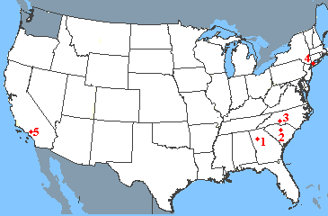
Suppose that you want to travel from Atlanta to Los Angeles, visiting your friends along the way. Unfortunately your friends live only on the eastern and western coasts, leading to a somewhat unconventional journey.

| Start | Destination | Miles |
|---|---|---|
| 1: Atlanta, GA | 2: Columbia, SC | 210 |
| 2: Columbia, SC | 3. Charlotte, NC | 90 |
| 3: Charlotte, NC | 4. New York, NY | 620 |
| 4. New York, NY | 5. Los Angeles, CA | 2790 |
- The number-average of the miles traveled in the four legs of the journey is 928 miles. This is the average distance travelled in each leg of the journey. It places equal emphasis on each leg.
- The mass-average of the miles traveled in the four legs of the journey is 2216 miles. This average places a greater emphasis on the leg of the journey with the largest "mass" - that is the fourth leg in which you travel 2790 miles. It is more representative of the major part of your journey.
- This mass-average/number-average ratio for this journey is 2.4, indicating that the trip is polydisperse with widely different mileages for the separate legs of the journey.
Viscosity Average
One of the oldest methods of measuring the average molecular weight of polymers is by solution viscosity. The viscosity-average molecular weight, \(\overline{M}_v\), lies somewhere between the number average and the weight average.
Chain Entanglement
Small molecules, even relatively large hydrocarbons such as the paraffins, do not have long enough chains to become entangled and do not exhibit polymer properties. Polymer molecules are long chains, which can become entangled with one another. Along with intermolecular forces, chain entanglement is an important factor contributing to the unique physical properties of polymers. The difficulty in untangling their chains makes polymers strong and resilient.
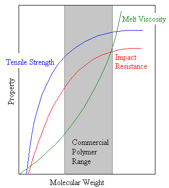
At some critical degree of polymerization a polymer will begin to show the mechanical properties, such as strength and toughness, that are characteristic of polymers. The value of the critical degree of polymerization that is necessary for a oligomer to show polymer properties is dependent on the intermolecular forces between polymer chains and on the amount of chain entanglement. All polymers exhibit no strength below DP = 30. The strength also does not change much above DP's in the 600 range. As the chains become very long, molecular entanglements and intermolecular forces become so great that the chains no longer slip along each other. At this point, further lengthening of the chains doesn't make much difference22.
Threshold Molecular Weight
Polymer chemists sometimes refer to the threshold molecular weight below which an oligomer will not display the properties needed for a particular application. The value of the threshold molecular weight depends on the application. If the polymer is to be used as an adhesive, the required molecular weight may be relatively low. If the polymer is to be used in a trash barrel on the other hand, a high molecular weight is required.
Beyond the critical degree of polymerization, as molecular weight grows larger polymer strength increases rapidly. Eventually, as is shown in the diagram at the right, the strength levels off.
The threshold molecular weight is a lower limit for the molecular weight required for a given commercial application. As the molecular weight increases the chains also entangle more, which increases the viscosity of the polymer melt. In most industrial applications a polymer is melted as it is processed so that it will flow into a mold or through an orifice. Eventually the viscosity gets so high that the polymer cannot be processed easily, establishing an upper molecular weight beyond which it is prohibitively expensive to process the polymer.

Thus we see that for a particular application only a certain molecular weight range is practical for a given polymer. This range is a compromise between optimum properties and ease of processing. Most of the practically useful polymers have a DP between 200 to 2000, corresponding to a molecular weight range from 20,000 to 200,000.
Contributors and Attributions
David Whisnant (Wofford College). Partial support for this work was provided by the National Science Foundation's Division of Undergraduate Education through grants DUE #9950809 and DUE #9950296. Additional support was provided by the Camille and Henry Dreyfus Foundation.


