12.4: Multi-Body General Planar Motion

Last updated
Save as PDF

Page ID: 54796

\( \newcommand{\vecs}[1]{\overset { \scriptstyle \rightharpoonup} {\mathbf{#1}} } \) \( \newcommand{\vecd}[1]{\overset{-\!-\!\rightharpoonup}{\vphantom{a}\smash {#1}}} \)\(\newcommand{\id}{\mathrm{id}}\) \( \newcommand{\Span}{\mathrm{span}}\) \( \newcommand{\kernel}{\mathrm{null}\,}\) \( \newcommand{\range}{\mathrm{range}\,}\) \( \newcommand{\RealPart}{\mathrm{Re}}\) \( \newcommand{\ImaginaryPart}{\mathrm{Im}}\) \( \newcommand{\Argument}{\mathrm{Arg}}\) \( \newcommand{\norm}[1]{\| #1 \|}\) \( \newcommand{\inner}[2]{\langle #1, #2 \rangle}\) \( \newcommand{\Span}{\mathrm{span}}\) \(\newcommand{\id}{\mathrm{id}}\) \( \newcommand{\Span}{\mathrm{span}}\) \( \newcommand{\kernel}{\mathrm{null}\,}\) \( \newcommand{\range}{\mathrm{range}\,}\) \( \newcommand{\RealPart}{\mathrm{Re}}\) \( \newcommand{\ImaginaryPart}{\mathrm{Im}}\) \( \newcommand{\Argument}{\mathrm{Arg}}\) \( \newcommand{\norm}[1]{\| #1 \|}\) \( \newcommand{\inner}[2]{\langle #1, #2 \rangle}\) \( \newcommand{\Span}{\mathrm{span}}\)\(\newcommand{\AA}{\unicode[.8,0]{x212B}}\)

In cases where multiple connected rigid bodies are undergoing some sort of motion, we can extend our analysis of general planar motion to this multi-body situation. In these cases, which we will call multi-body kinetics problems, we will analyze each body independently as we did for general planar motion, but we will also need to pay attention to the Newton's Third Law pairs. Each body will have forces exerted on it by the surrounding bodies, and it will exert equal and opposite forces back through those same connections.

A group of robotic arms work on assembling the skeleton of a vehicle. — Figure \(\PageIndex{1}\): These robotic arms are a good example of a multi-body kinetics problem. As one section of the arm accelerates, it will exert forces on the other arm sections it is connected to. Image by Chris Chesher, CC-BY-NC-SA 2.0.

To analyze a multi-body system, we will start by drawing a free body diagram of each body in motion. Be sure to identify the center of mass, as well as identifying all known and unknown forces, and known and unknown moments acting on the body. When drawing forces at connection points, be sure to make the forces equal and opposite on the connected body to satisfy Newton's Third Law. It is also sometimes helpful to label any key dimensions as well as using dashed lines to identify any known accelerations or angular accelerations. Often, you will need to solve a kinematics problem using absolute motion analysis or relative motion analysis in order to determine the accelerations of the centers of mass and the angular accelerations for each body. Make sure all these accelerations are with respect to ground.

Next we move onto identifying the equations of motion for each body in the system. In two dimensions, we will use the same three equations we used for general planar motion. Be sure to find the the accelerations of all the centers of masses, find all moments about the center of mass, and take the mass moments of inertia about the center of mass of each body.

\[ \sum F_x = m * a_x \]

\[ \sum F_y = m * a_y \]

\[ \sum M_G = I_G * \alpha \]

Plugging the known forces, moments, and accelerations into the above equations we can solve for up to three unknowns per body. If more than three unknowns exist in any one set of equations, you will need to start with an adjacent body. Once unknown forces are determined on one body, they can become knowns on the connected body, reducing the number of unknowns to solve for.

Video lecture covering this section, delivered by Dr. Jacob Moore. YouTube source: https://youtu.be/-tAP08srNrU.

Example \(\PageIndex{1}\)

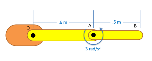
A robotic arm has two sections (OA and AB), with section OA having a mass of 10 kg and section AB having a mass of 7 kg. Treat each section as a slender rod. If we wish to accelerate member AB from a standstill at a rate of 3 rad/s² and keep the left section stationary, what moments must we exert at joints O and A?

A two-segment robotic arm consists of one 0.6-meter-long segment, where the left endpoint O is attached to a stationary base and the right endpoint A is attached to a 0.5-meter-long segment AB. Both segments are horizontal. At point A, a counterclockwise rotation is shown, with an angular acceleration of 3° rad/s. — Figure \(\PageIndex{2}\): problem diagram for Example \(\PageIndex{1}\). A robotic arm consists of two segments that are currently horizontal, with the left end of the left segment being attached to a base and the right segment undergoing angular acceleration.

Solution: Video \(\PageIndex{2}\): Worked solution to example problem \(\PageIndex{1}\), provided by Dr. Majid Chatsaz. YouTube source: https://youtu.be/zR_uhVM1uH0.