
Chapter 1: Measurement Processes and Confidence Intervals
- Page ID
- 116466

\( \newcommand{\vecs}[1]{\overset { \scriptstyle \rightharpoonup} {\mathbf{#1}} } \)
\( \newcommand{\vecd}[1]{\overset{-\!-\!\rightharpoonup}{\vphantom{a}\smash {#1}}} \)
\( \newcommand{\dsum}{\displaystyle\sum\limits} \)
\( \newcommand{\dint}{\displaystyle\int\limits} \)
\( \newcommand{\dlim}{\displaystyle\lim\limits} \)
\( \newcommand{\id}{\mathrm{id}}\) \( \newcommand{\Span}{\mathrm{span}}\)
( \newcommand{\kernel}{\mathrm{null}\,}\) \( \newcommand{\range}{\mathrm{range}\,}\)
\( \newcommand{\RealPart}{\mathrm{Re}}\) \( \newcommand{\ImaginaryPart}{\mathrm{Im}}\)
\( \newcommand{\Argument}{\mathrm{Arg}}\) \( \newcommand{\norm}[1]{\| #1 \|}\)
\( \newcommand{\inner}[2]{\langle #1, #2 \rangle}\)
\( \newcommand{\Span}{\mathrm{span}}\)
\( \newcommand{\id}{\mathrm{id}}\)
\( \newcommand{\Span}{\mathrm{span}}\)
\( \newcommand{\kernel}{\mathrm{null}\,}\)
\( \newcommand{\range}{\mathrm{range}\,}\)
\( \newcommand{\RealPart}{\mathrm{Re}}\)
\( \newcommand{\ImaginaryPart}{\mathrm{Im}}\)
\( \newcommand{\Argument}{\mathrm{Arg}}\)
\( \newcommand{\norm}[1]{\| #1 \|}\)
\( \newcommand{\inner}[2]{\langle #1, #2 \rangle}\)
\( \newcommand{\Span}{\mathrm{span}}\) \( \newcommand{\AA}{\unicode[.8,0]{x212B}}\)
\( \newcommand{\vectorA}[1]{\vec{#1}} % arrow\)
\( \newcommand{\vectorAt}[1]{\vec{\text{#1}}} % arrow\)
\( \newcommand{\vectorB}[1]{\overset { \scriptstyle \rightharpoonup} {\mathbf{#1}} } \)
\( \newcommand{\vectorC}[1]{\textbf{#1}} \)
\( \newcommand{\vectorD}[1]{\overrightarrow{#1}} \)
\( \newcommand{\vectorDt}[1]{\overrightarrow{\text{#1}}} \)
\( \newcommand{\vectE}[1]{\overset{-\!-\!\rightharpoonup}{\vphantom{a}\smash{\mathbf {#1}}}} \)
\( \newcommand{\vecs}[1]{\overset { \scriptstyle \rightharpoonup} {\mathbf{#1}} } \)
\(\newcommand{\longvect}{\overrightarrow}\)
\( \newcommand{\vecd}[1]{\overset{-\!-\!\rightharpoonup}{\vphantom{a}\smash {#1}}} \)
\(\newcommand{\avec}{\mathbf a}\) \(\newcommand{\bvec}{\mathbf b}\) \(\newcommand{\cvec}{\mathbf c}\) \(\newcommand{\dvec}{\mathbf d}\) \(\newcommand{\dtil}{\widetilde{\mathbf d}}\) \(\newcommand{\evec}{\mathbf e}\) \(\newcommand{\fvec}{\mathbf f}\) \(\newcommand{\nvec}{\mathbf n}\) \(\newcommand{\pvec}{\mathbf p}\) \(\newcommand{\qvec}{\mathbf q}\) \(\newcommand{\svec}{\mathbf s}\) \(\newcommand{\tvec}{\mathbf t}\) \(\newcommand{\uvec}{\mathbf u}\) \(\newcommand{\vvec}{\mathbf v}\) \(\newcommand{\wvec}{\mathbf w}\) \(\newcommand{\xvec}{\mathbf x}\) \(\newcommand{\yvec}{\mathbf y}\) \(\newcommand{\zvec}{\mathbf z}\) \(\newcommand{\rvec}{\mathbf r}\) \(\newcommand{\mvec}{\mathbf m}\) \(\newcommand{\zerovec}{\mathbf 0}\) \(\newcommand{\onevec}{\mathbf 1}\) \(\newcommand{\real}{\mathbb R}\) \(\newcommand{\twovec}[2]{\left[\begin{array}{r}#1 \\ #2 \end{array}\right]}\) \(\newcommand{\ctwovec}[2]{\left[\begin{array}{c}#1 \\ #2 \end{array}\right]}\) \(\newcommand{\threevec}[3]{\left[\begin{array}{r}#1 \\ #2 \\ #3 \end{array}\right]}\) \(\newcommand{\cthreevec}[3]{\left[\begin{array}{c}#1 \\ #2 \\ #3 \end{array}\right]}\) \(\newcommand{\fourvec}[4]{\left[\begin{array}{r}#1 \\ #2 \\ #3 \\ #4 \end{array}\right]}\) \(\newcommand{\cfourvec}[4]{\left[\begin{array}{c}#1 \\ #2 \\ #3 \\ #4 \end{array}\right]}\) \(\newcommand{\fivevec}[5]{\left[\begin{array}{r}#1 \\ #2 \\ #3 \\ #4 \\ #5 \\ \end{array}\right]}\) \(\newcommand{\cfivevec}[5]{\left[\begin{array}{c}#1 \\ #2 \\ #3 \\ #4 \\ #5 \\ \end{array}\right]}\) \(\newcommand{\mattwo}[4]{\left[\begin{array}{rr}#1 \amp #2 \\ #3 \amp #4 \\ \end{array}\right]}\) \(\newcommand{\laspan}[1]{\text{Span}\{#1\}}\) \(\newcommand{\bcal}{\cal B}\) \(\newcommand{\ccal}{\cal C}\) \(\newcommand{\scal}{\cal S}\) \(\newcommand{\wcal}{\cal W}\) \(\newcommand{\ecal}{\cal E}\) \(\newcommand{\coords}[2]{\left\{#1\right\}_{#2}}\) \(\newcommand{\gray}[1]{\color{gray}{#1}}\) \(\newcommand{\lgray}[1]{\color{lightgray}{#1}}\) \(\newcommand{\rank}{\operatorname{rank}}\) \(\newcommand{\row}{\text{Row}}\) \(\newcommand{\col}{\text{Col}}\) \(\renewcommand{\row}{\text{Row}}\) \(\newcommand{\nul}{\text{Nul}}\) \(\newcommand{\var}{\text{Var}}\) \(\newcommand{\corr}{\text{corr}}\) \(\newcommand{\len}[1]{\left|#1\right|}\) \(\newcommand{\bbar}{\overline{\bvec}}\) \(\newcommand{\bhat}{\widehat{\bvec}}\) \(\newcommand{\bperp}{\bvec^\perp}\) \(\newcommand{\xhat}{\widehat{\xvec}}\) \(\newcommand{\vhat}{\widehat{\vvec}}\) \(\newcommand{\uhat}{\widehat{\uvec}}\) \(\newcommand{\what}{\widehat{\wvec}}\) \(\newcommand{\Sighat}{\widehat{\Sigma}}\) \(\newcommand{\lt}{<}\) \(\newcommand{\gt}{>}\) \(\newcommand{\amp}{&}\) \(\definecolor{fillinmathshade}{gray}{0.9}\)Lecture 1: Measurement Processes and Confidence Intervals
Topics Covered in this Class
Part I: Measurements, Confidence Intervals, T-Tests, P-Values, ANOVA, Fourier Analysis, Wheatstone Bridges
Part II: Laplace Transforms, Stability, Feedback Control, Root Locus, Routh-Hurwitz, Bode Plots, Control Design, PID Control, Nyquist Plots
What is a Measurement?
A measurement is a quantitative comparison between a predefined standard and a measurand.
What are some examples of different types of measurements we can make?
• Temperature
• Length
• Time
• Stress
• Strain
• Viscosity
• Force
• Torque
• ....
The process or act of measurement is a quantitative comparison between a predefined standard and a measurand.
Measurand: the particular physical parameter being observed and quantified, i.e., the input quantity of the measuring process
Standard: Must be of the same character as the measurand and usually recognized by the NIST (National Institute of Standards and Technology)
What are some standards?
• Tape Measure
• Balance
• Speed of Light
• ...
The act of measurement produces a result.
ADD FIGURE
The significance of measurements:
• Obtain quantitative information on the actual state of physical variables and processes (i.e. T, P, V, etc.)
• Vital for control processes which require measured discrepancy between actual and desired output (i.e. temperature control on sheet annealing line)
• Daily operations (i.e. central power station)
• Establishing costs
Measurements are only useful if they are reliable. This brings up the concept of the accuracy or uncertainty of a measurement. No measurement is perfect and therefore engineers must place tolerances on measured values.
There are two basic methods of measurement: i) direct and ii) indirect
Direct Comparison:
• Measurements utilize a primary or secondary standard
• Ex: Measuring length using tape measure, which is a secondary standard, primary standard would use speed of light
• Simple measurement however often we need greater accuracy
• Direct comparison is less common than indirect comparison
Indirect Comparison:
• Utilizes some form of transducing device coupled to a chain of connecting apparatus as the measuring system
• Input or measurand converted into an analogous form which is a necessary conversion so the information is intelligible
• Ex. Human senses cannot detect strain so conversion is necessary
• The analogous signal is processed and can be amplified, filtered, or remotely recorded
• Transducers convert mechanical input into analogous electrical for processing, particularly for dynamic mechanical measurements
Generalized Measuring System
Stage I: Detection-transduction or sensor-transducer stage
Stage II: Intermediate or signal-conditioning stage
Stage III: Terminating or readout-recording stage
ADD FIGURE
Examples:
• Stage I: spring-mass, thermocouple, piezoelectric
• Stage II: gearing, dashpots, bridges, filters
• Stage III: liquid column, digital printout, magnetic recording
Stage 1: Sensor-Transducer Stage
• Primary function is to detect or sense the measurand
• Ideally should be insensitive to all other inputs, ex. insensitive to temperature for strain gauge
• Unwanted sensitivity can lead to error termed noise when it varies rapidly and drift when it varies slowly
Stage 2: Signal-Conditioning Stage
• Primary purpose is to modify the transduced information so it is acceptable to Stage 3
• The transduced signal is conditioned via amplification, filtering, integration, differentiation, etc.
Stage 3: Readout-Recording Stage
• Provides information in a form comprehensible to one of the human senses
• Example: Relative displacement or a digital readout
Ex. 1: Tire Pressure Gauge
ADD FIGURE
Task: Fill out the generalized block diagram for using a tire pressure gauge to measure tire pressure
What is the Measurand/Input?
- Pressure
What is the Sensor-Transducer?
- The piston-cylinder senses pressure and converts it to force. A secondary transducer (spring) converts the force to displacement.
What is the Signal Conditioner?
- None in this case.
What is the Readout-Recording?
- The displacement of the stem, which can be read from the calibrated scale.
Using Correct Terminology When Assessing Measurement Quality/Apparatus Performance
• Accuracy: Difference between measured and true values. Manufacturer will specify maximum error but not confidence intervals typically.
• Precision: Difference between reported values during repeated measurements of same quantity.
• Resolution: Smallest increment of change in the measured value that can be determined by the readout scale. Often the same as precision.
• Sensitivity: The change of an instrument’s output per unit change in the measured quantity. Higher sensitivity often indicates finer resolution, better precision, and higher accuracy.
Error and Uncertainty:
Error is the difference between the measured and true value of the quantity being measured. Unfortunately, the true value can never really be known so instead we quantify the uncertainty of a measurement at specific levels of confidence. Error can be categorized into two basic categories either bias or precision error/uncertainty. We will cover uncertainty and error analysis much more in-depth in the next several lectures...but never use percent error in this course.
Error
We can begin with our discussion of error by defining the following equation
\begin{equation}
Error = x_{m} - x_{true}
\end{equation}
where \(x_m\) is the measured value and \(x_{true}\) is the true value.
When designing an experimental system or executing an experiment the experimentalist’s primary objective should be to minimize the error. After the experiment is completed we need to estimate a bound on the error with a degree of certainty or a confidence interval (i.e. 90%, 95%, 99%), hopefully you have encountered confidence intervals before but if not no worries we will discuss this in depth.
There are many different sources of inaccuracy or error however most errors can be classified as:
(1) Precision
(2) Bias
(3) Illegitimate
(4) Errors that are sometimes bias or sometimes precision errors
In this course we will spend a considerable amount of time discussing 1. Precision and 2. Bias error in great detail. But we will discuss all these sources of error and how to account for them when designing experiments or presenting your results. Let’s start with Precision Error.
Precision or Random Errors
I really do not like the term random error but you will occasionally see that term in literature but in this course we will use the term precision primarily.
Precision errors are different for each successive measurement. Thus if you create a histogram, which shows the probability of encountering or measuring a specific measurand, the width of your distribution (hopefully it is Gaussian) will be due to precision error if that is the only source of error in your experiment. From this distribution, statistical analysis can be utilized to estimate the size of the precision error. Typically bias and precision errors occur simultaneously and contributes to the total error, more on this fun calculation later, hope you remember Taylor expansions....
Why Do We Have Precision Error?
(1) Disturbances to the equipment
(2) Fluctuating experimental conditions
(3) Insufficient measuring-system sensitivity
(4) Stochastic (Random) nature of measurements even in static conditions
Examples of Precision Error:
• Measuring temperature with thermocouple as temperature fluctuates
• Measure the length of a beam with a micrometer you will get slightly different measurements than classmates
• Changes in temperature conditions can affect swimming of bacteria
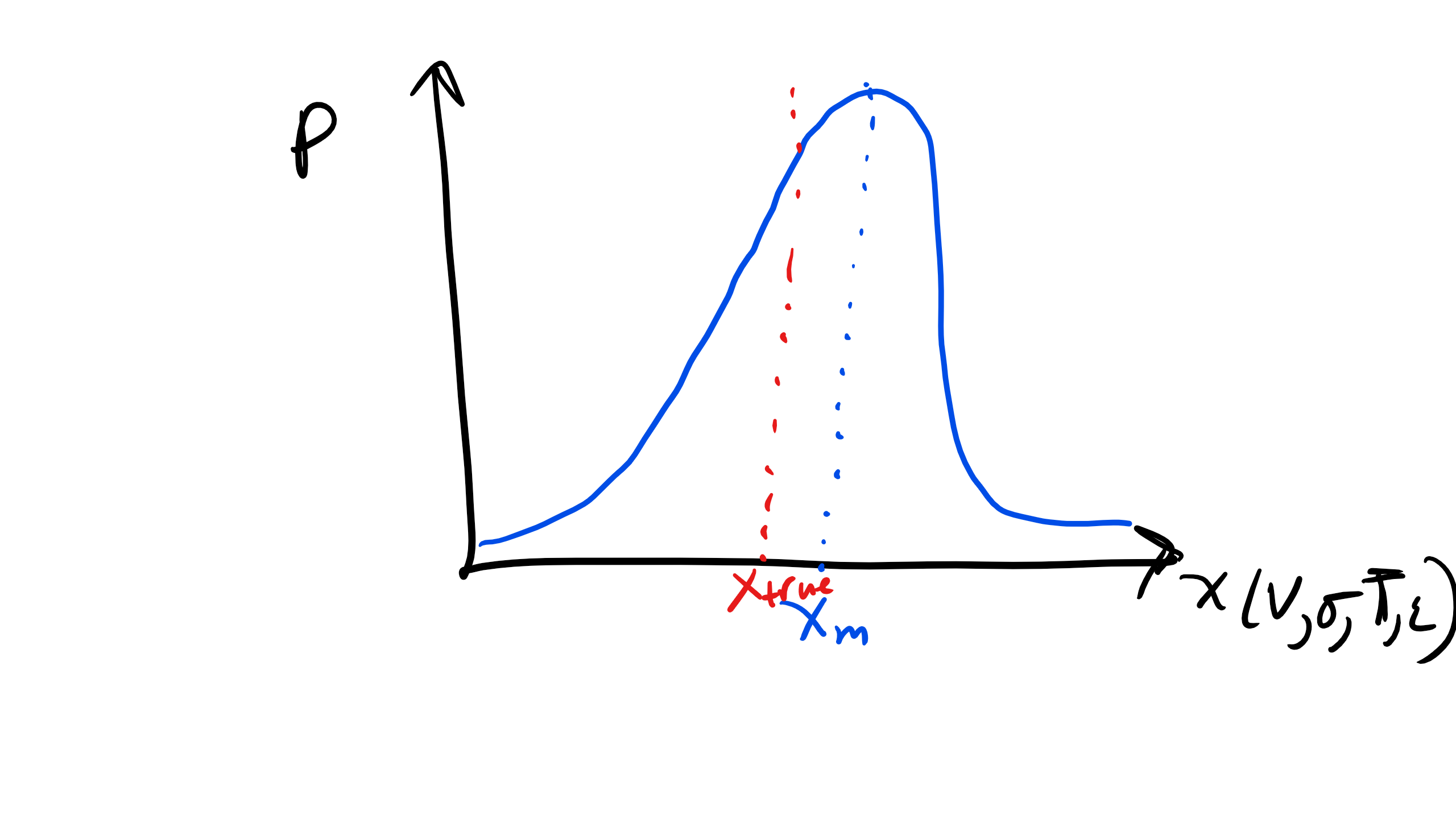 Figure \(\PageIndex{1}\): Precision Error Distribution.
Bias or Systematic Errors
I like the term bias and systematic much better than random. However, in this course we will primarily use the term Bias error.
Bias errors will occur the same way each time a measurement is made. For example a balance that consistently reads 0.5 mg heavier. In some literature you might see this termed as a fixed offset error. The key thing to note about bias errors is they are fixed and thus they do not show a distribution. This is in stark contrast to precision errors which show a distribution, typically Gaussian. Therefore if there is no distribution we cannot apply any statistical analysis.
There are multiple types of bias errors:
(1) Calibration errors
• This is the most common error
• Typically calibration errors are zero-offset errors which cause all read- ing to be offset by constant amount or scale errors
• I.e. scale constantly light by 1lb or clock runs fast by 1 minute
• Can be reduced via calibration procedures and proving the system via comparison with known standard
(2) Consistently recurring human errors
• Ex. experimenter who consistently jumps the gun when recording synchronized readings either time, voltage, etc.
(3) Errors caused by defective equipment
(4) Loading errors
• i.e. not putting a DSC pan at the center of the DSC will skew temperature measurements
(5) System resolution limits
• i.e. Bias error for a ruler with cm tick marks will be cm, compared to a micrometer with 1µm resolution, that is 4 order of magnitude difference.
Illegitimate Error
Illegitimate error can and most likely will occur to you at some point as you perform experiments as an engineer. Illegitimate errors include
• Blunders and mistakes
• Computational or calculation errors
• Analysis errors
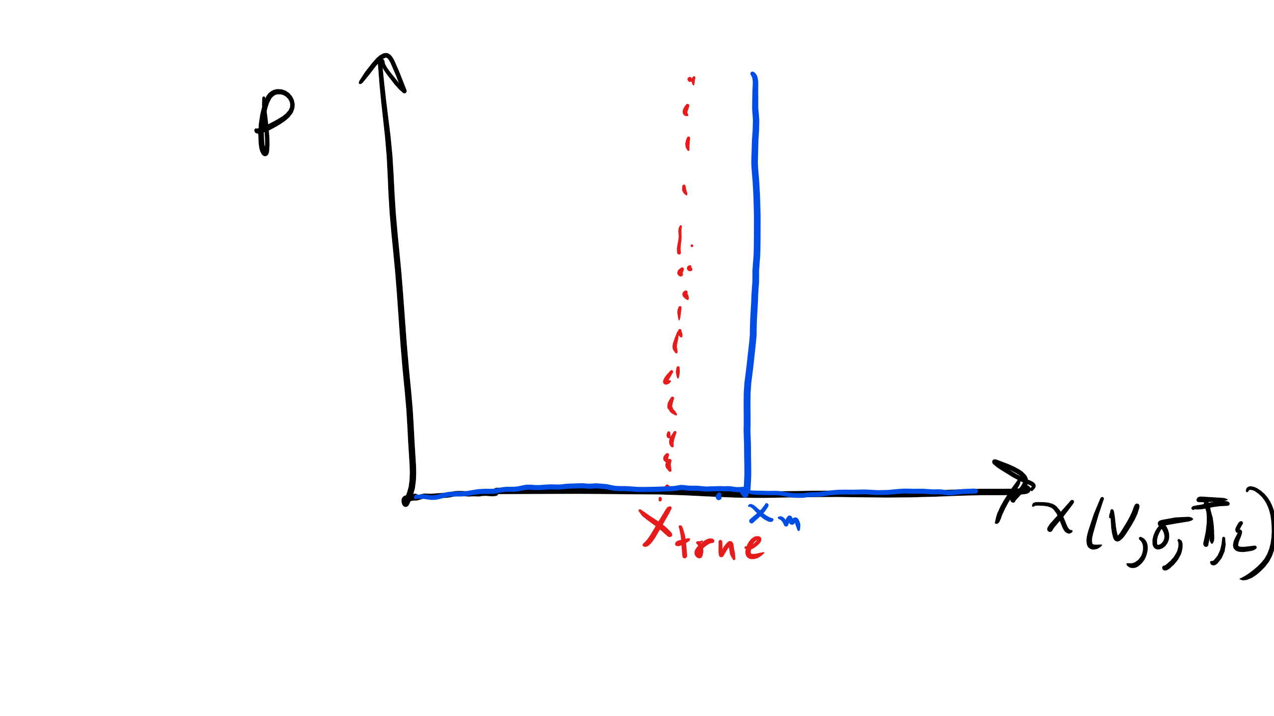 Figure \(\PageIndex{2}\): Bias Error Distribution
While these things can occur in lab you must always perform the experiment again. You cannot simply present your results in either a presentation or a form of technical writing and attribute error to illegitimate error. You must perform the experiment again.
Errors That Are Sometimes Bias and Sometimes Precision Error:
These are the most difficult sources of error that we must analyze as it is difficult to determine what type of error analysis must be done and which error has a distribution and what does not.
• Instrument Hysteresis
– Hysteresis error can be seen in stress strain measurements and is path dependent
• Calibration drift and variation in test or environmental conditions
– Drift occurs when the response varies over time often due to sensitivity to temperature or humidity
• Variations in procedure or definition among experimenters
Quantifying Total Uncertainty, Comprehensive Error Analysis
Again typically we are concerned with bias and precision error when evaluating experimental data. And this data comes from two classes of experiments: i) single- sample and ii) repeated-sample experiments.
A sample refers to an individual measurement of a specific quantity. Ex. Measuring strain in a material several times under identical loading is a repeated-sample experiment. A single measurement of strain is a single-sample experiment and we cannot extract the distribution of precision error in this case. In this course and in your career as an engineer you will most likely be taking multiple measurements,
i.e. repeated sample experiments. Single sample experiments are more uncommon and typically occur when the measurement you are making is extremely difficult and multiple experiments are non realistic to conduct, typically due to economic or practicality reasons.
The total uncertainty \(U_x\) in a measurement of x is
\begin{equation}
U_{x} = \sqrt{B_{x}^2 + P_{x}^2}
\end{equation}
where \(B_x\) if the bias uncertainty in a measurement of x and \(P_x\) is the precision uncertainty. Note that x is just a variable and we can talk about uncertainty in measuring volume (V), pressure (P), stress (σ), etc.
This is a largely empirically derived formula however it does depend on the assump-tion that the bias and precision uncertainty are independent sources of error. Also the bias and precision uncertainty should have the same confidence level when calculating the total uncertainty. We will come back to this a bit later in excruciating detail for this calculation so please be patient.
Minimizing Error in Designing Experiments
Best time to minimize experimental error is in the design stage. You should perform a single-sample uncertainty analysis of the proposed experimental arrangement prior to building the apparatus. This allows one to make a decision on whether the expected uncertainty is acceptable and to identify the sources of uncertainty. So when designing an experiment:
• Avoid approaches that require two large numbers to be measured to determine the small difference between them
• Design experiments or sensors that amplify the signal strength to improve sensitivity
• Build null designs in which the output is measured as a change from zero rather than as a change in nonzero value
• Avoid experiments with large correction factors must be applied as part of the data-reduction procedure
• Attempt to minimize the influence of the measuring system on the measured variable
• Calibrate entire system to minimize calibration related bias errors.
Gaussian and Normal Distribution
One of the most common distributions encountered is the Gaussian distribution, also called the normal distribution or bell curve.
The Gaussian distribution describes an infinite population of data where each datum represents a measurement of a single quantity. Each value x differs due to precision error.
The probability of obtaining a specific value x is described by the probability density function (PDF), f(x).
The total area under the curve equals 1, which represents 100% probability:
\[P = \int_{-\infty}^{\infty} f(x)\, dx = 1\]
Gaussian PDF:
\[f(x) = \frac{1}{\sigma \sqrt{2\pi}} \exp\left( -\frac{(x - \mu)^2}{2\sigma^2} \right)\]
Where \(\mu\) = population mean and \(\sigma\) = population standard deviation.
To simplify, define \[z = \frac{x - \mu}{\sigma)}\], so:
\[f(z) = \frac{1}{\sqrt{2 \pi)}} e^{-z^2/2}\]

You can use Z-tables to find the area under the curve for a given z. For example, the 95% confidence interval contains most values within ±1.96\(\sigma\).
Outliers
Outliers are data points that are much higher or lower than the mean.
You can disregard a data point if it exceeds 3\(\sigma\), but must report it and justify its exclusion.
Confidence Intervals
The area between ±z under the standard curve defines a confidence interval.
Example: A 95% confidence interval covers ~95% of the population's measurements.
Example Problems - Confidence Intervals
Working with Z Tables
• What is the area under the standard normal distribution curve between z = -1.43 and z = 1.43?
• What percent of the population lies within this range?
• What range of z contains 90% of the data?
Running and Tumbling E. coli
Given: mean = 3 \(\mu\)m/s, \(\sigma\) = 0.1 \(\mu\)m/s, range = [2.857, 3.143] \(\mu\)m/s
• Assume normal distribution
• Compute z for bounds
• Use standard normal table to compute area
• Estimate number of samples within range
• Determine 95% confidence bounds
Marble Diameters
Given: N = 765 marbles, \(\mu\) = 200 mm, \(\sigma\) = 20 mm
• Determine diameter range for 60% of marbles
Ultimate Tensile Strength Measurements
Given: \(\mu\) = 303 MPa, \(\sigma\) = 33 MPa
• What is the probability a sample exceeds 350 MPa?
Voltage Measurements
Given: \(\mu\) = 10 V, \(\sigma\) = 3.4 V
• How many of 150 measurements fall between 10–15 V?
Under Pressure Measurements
Given: \(\mu\) = 39 Pa, \(\sigma\) = 4 Pa, N = 120
• How many measurements fall between 35–45 Pa?
• How many below 35 Pa?
• How many below 45 Pa?