
Chapter 10: System
- Page ID
- 123786

\( \newcommand{\vecs}[1]{\overset { \scriptstyle \rightharpoonup} {\mathbf{#1}} } \)
\( \newcommand{\vecd}[1]{\overset{-\!-\!\rightharpoonup}{\vphantom{a}\smash {#1}}} \)
\( \newcommand{\dsum}{\displaystyle\sum\limits} \)
\( \newcommand{\dint}{\displaystyle\int\limits} \)
\( \newcommand{\dlim}{\displaystyle\lim\limits} \)
\( \newcommand{\id}{\mathrm{id}}\) \( \newcommand{\Span}{\mathrm{span}}\)
( \newcommand{\kernel}{\mathrm{null}\,}\) \( \newcommand{\range}{\mathrm{range}\,}\)
\( \newcommand{\RealPart}{\mathrm{Re}}\) \( \newcommand{\ImaginaryPart}{\mathrm{Im}}\)
\( \newcommand{\Argument}{\mathrm{Arg}}\) \( \newcommand{\norm}[1]{\| #1 \|}\)
\( \newcommand{\inner}[2]{\langle #1, #2 \rangle}\)
\( \newcommand{\Span}{\mathrm{span}}\)
\( \newcommand{\id}{\mathrm{id}}\)
\( \newcommand{\Span}{\mathrm{span}}\)
\( \newcommand{\kernel}{\mathrm{null}\,}\)
\( \newcommand{\range}{\mathrm{range}\,}\)
\( \newcommand{\RealPart}{\mathrm{Re}}\)
\( \newcommand{\ImaginaryPart}{\mathrm{Im}}\)
\( \newcommand{\Argument}{\mathrm{Arg}}\)
\( \newcommand{\norm}[1]{\| #1 \|}\)
\( \newcommand{\inner}[2]{\langle #1, #2 \rangle}\)
\( \newcommand{\Span}{\mathrm{span}}\) \( \newcommand{\AA}{\unicode[.8,0]{x212B}}\)
\( \newcommand{\vectorA}[1]{\vec{#1}} % arrow\)
\( \newcommand{\vectorAt}[1]{\vec{\text{#1}}} % arrow\)
\( \newcommand{\vectorB}[1]{\overset { \scriptstyle \rightharpoonup} {\mathbf{#1}} } \)
\( \newcommand{\vectorC}[1]{\textbf{#1}} \)
\( \newcommand{\vectorD}[1]{\overrightarrow{#1}} \)
\( \newcommand{\vectorDt}[1]{\overrightarrow{\text{#1}}} \)
\( \newcommand{\vectE}[1]{\overset{-\!-\!\rightharpoonup}{\vphantom{a}\smash{\mathbf {#1}}}} \)
\( \newcommand{\vecs}[1]{\overset { \scriptstyle \rightharpoonup} {\mathbf{#1}} } \)
\(\newcommand{\longvect}{\overrightarrow}\)
\( \newcommand{\vecd}[1]{\overset{-\!-\!\rightharpoonup}{\vphantom{a}\smash {#1}}} \)
\(\newcommand{\avec}{\mathbf a}\) \(\newcommand{\bvec}{\mathbf b}\) \(\newcommand{\cvec}{\mathbf c}\) \(\newcommand{\dvec}{\mathbf d}\) \(\newcommand{\dtil}{\widetilde{\mathbf d}}\) \(\newcommand{\evec}{\mathbf e}\) \(\newcommand{\fvec}{\mathbf f}\) \(\newcommand{\nvec}{\mathbf n}\) \(\newcommand{\pvec}{\mathbf p}\) \(\newcommand{\qvec}{\mathbf q}\) \(\newcommand{\svec}{\mathbf s}\) \(\newcommand{\tvec}{\mathbf t}\) \(\newcommand{\uvec}{\mathbf u}\) \(\newcommand{\vvec}{\mathbf v}\) \(\newcommand{\wvec}{\mathbf w}\) \(\newcommand{\xvec}{\mathbf x}\) \(\newcommand{\yvec}{\mathbf y}\) \(\newcommand{\zvec}{\mathbf z}\) \(\newcommand{\rvec}{\mathbf r}\) \(\newcommand{\mvec}{\mathbf m}\) \(\newcommand{\zerovec}{\mathbf 0}\) \(\newcommand{\onevec}{\mathbf 1}\) \(\newcommand{\real}{\mathbb R}\) \(\newcommand{\twovec}[2]{\left[\begin{array}{r}#1 \\ #2 \end{array}\right]}\) \(\newcommand{\ctwovec}[2]{\left[\begin{array}{c}#1 \\ #2 \end{array}\right]}\) \(\newcommand{\threevec}[3]{\left[\begin{array}{r}#1 \\ #2 \\ #3 \end{array}\right]}\) \(\newcommand{\cthreevec}[3]{\left[\begin{array}{c}#1 \\ #2 \\ #3 \end{array}\right]}\) \(\newcommand{\fourvec}[4]{\left[\begin{array}{r}#1 \\ #2 \\ #3 \\ #4 \end{array}\right]}\) \(\newcommand{\cfourvec}[4]{\left[\begin{array}{c}#1 \\ #2 \\ #3 \\ #4 \end{array}\right]}\) \(\newcommand{\fivevec}[5]{\left[\begin{array}{r}#1 \\ #2 \\ #3 \\ #4 \\ #5 \\ \end{array}\right]}\) \(\newcommand{\cfivevec}[5]{\left[\begin{array}{c}#1 \\ #2 \\ #3 \\ #4 \\ #5 \\ \end{array}\right]}\) \(\newcommand{\mattwo}[4]{\left[\begin{array}{rr}#1 \amp #2 \\ #3 \amp #4 \\ \end{array}\right]}\) \(\newcommand{\laspan}[1]{\text{Span}\{#1\}}\) \(\newcommand{\bcal}{\cal B}\) \(\newcommand{\ccal}{\cal C}\) \(\newcommand{\scal}{\cal S}\) \(\newcommand{\wcal}{\cal W}\) \(\newcommand{\ecal}{\cal E}\) \(\newcommand{\coords}[2]{\left\{#1\right\}_{#2}}\) \(\newcommand{\gray}[1]{\color{gray}{#1}}\) \(\newcommand{\lgray}[1]{\color{lightgray}{#1}}\) \(\newcommand{\rank}{\operatorname{rank}}\) \(\newcommand{\row}{\text{Row}}\) \(\newcommand{\col}{\text{Col}}\) \(\renewcommand{\row}{\text{Row}}\) \(\newcommand{\nul}{\text{Nul}}\) \(\newcommand{\var}{\text{Var}}\) \(\newcommand{\corr}{\text{corr}}\) \(\newcommand{\len}[1]{\left|#1\right|}\) \(\newcommand{\bbar}{\overline{\bvec}}\) \(\newcommand{\bhat}{\widehat{\bvec}}\) \(\newcommand{\bperp}{\bvec^\perp}\) \(\newcommand{\xhat}{\widehat{\xvec}}\) \(\newcommand{\vhat}{\widehat{\vvec}}\) \(\newcommand{\uhat}{\widehat{\uvec}}\) \(\newcommand{\what}{\widehat{\wvec}}\) \(\newcommand{\Sighat}{\widehat{\Sigma}}\) \(\newcommand{\lt}{<}\) \(\newcommand{\gt}{>}\) \(\newcommand{\amp}{&}\) \(\definecolor{fillinmathshade}{gray}{0.9}\)System Stability and Pole-Based Classification
System stability is directly tied to the locations of the poles of the transfer function \( H(s) = \frac{Y(s)}{U(s)} \). The classification is as follows:
Stable: all poles lie in the open left-half of the complex plane (LHP).
Marginally stable: poles on the imaginary axis, but all are simple (non-repeated).
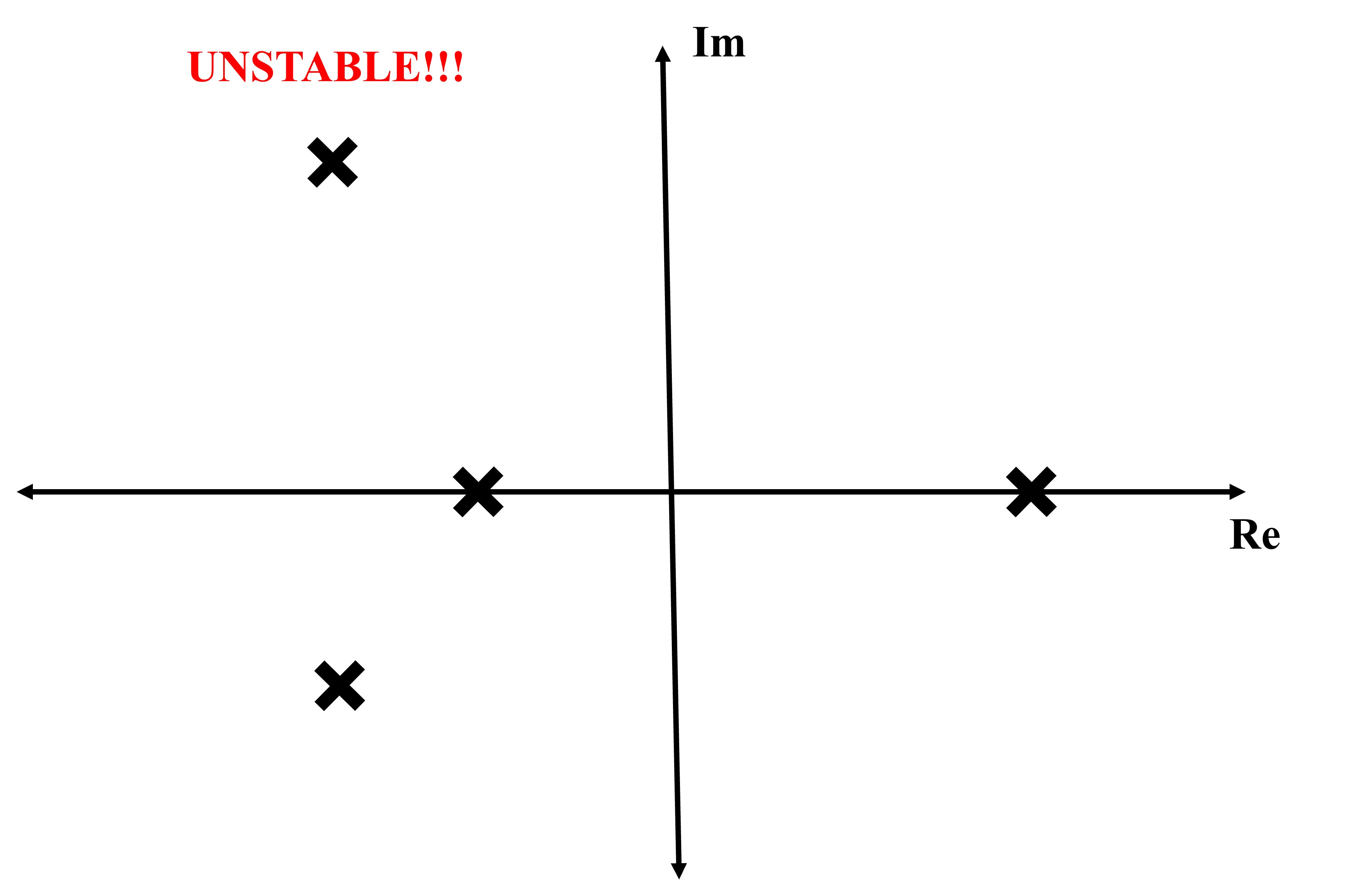
Unstable: at least one pole in the right-half plane (RHP), or repeated poles on the imaginary axis.
Worked Example: First-Order Impulse Response
Given:
\[
H(s) = \frac{1}{s + \sigma}, \quad \text{Impulse response: } y(t) = e^{-\sigma t}
\]
If \( \sigma > 0 \), \( y(t) \to 0 \): stable
If \( \sigma = 0 \), \( y(t) = 1 \): marginally stable
If \( \sigma < 0 \), \( y(t) \to \infty \): unstable
The most general definition of stability is that the plant or transfer function is stable if and only if the output function \( y(t) \) goes to zero as time goes to infinity. We are marginally stable if and only if the absolute value of \( y(t) \) is less than some constant value but also never decays to zero and the system is unstable if and only if \( y(t) \) goes to infinity as time goes to infinity.
Pole Stability Conditions
Let's consider a plant function \( P(s) \) with poles \( p_i \). Then we can summarize that:
P(s) is stable if and only if all \( p_i \) are in the LHP.
P(s) is marginally stable if and only if:
- All \( p_i \) are in the LHP or on the imaginary axis, and
- Some non-repeated \( p_i \) are on the imaginary axis.
P(s) is unstable if and only if:
- Some \( p_i \) are in the RHP, or
- Some \( p_i \) are on the imaginary axis and are repeated.
Let's look at some examples to test if they are stable:


We can also look at some transfer functions and determine if they are stable:
\[
\frac{1}{s+4}, \quad \frac{s-3}{(s+5)^2+2^2}, \quad \frac{1}{s-5}
\]
The first two transfer functions are stable. The last is unstable.
Stability for First Order Transfer Functions
\[
\frac{1}{s+a}
\]
We are stable as long as \( a > 0 \).
Stability for Second Order Transfer Functions
\[
\frac{1}{s^2 + a_1 s + a_2}
\]
We are stable as long as \( a_1 > 0 \) and \( a_2 > 0 \).
Stability for nth Order Transfer Functions
\[
\frac{1}{s^n + a_1 s^{n-1} + a_2 s^{n-2} + \dots + a_n}
\]
We are stable as long as all \( a_i > 0 \). However, this condition is not comprehensive enough to guarantee stability. To be rigorous for nth-order transfer functions, we must use the Routh-Hurwitz Stability Criterion.
The Routh-Hurwitz Stability Criterion
This technique provides a systematic method to determine the number of poles with positive real parts (i.e., unstable poles) without explicitly calculating roots. The method involves:
1. Writing the characteristic polynomial:
\[
P(s) = a_n s^n + a_{n-1}s^{n-1} + \cdots + a_0
\]
2. Constructing the Routh table using these coefficients.
3. Checking signs in the first column.
Stability condition: All entries in the first column must be strictly positive.
Interpretation:
The number of sign changes in the first column equals the number of RHP poles.
A zero in the first column requires special handling (epsilon substitution or auxiliary polynomial).
Assume \( a_0 > 0 \) for normalization. The Routh array is built row by row as follows:
Step 1: First Two Rows
Row 1 (even powers): \( a_0, a_2, a_4, \dots \)
Row 2 (odd powers): \( a_1, a_3, a_5, \dots \)
Step 2: Compute Subsequent Rows
Use the following formula for all subsequent elements:
\[
b_1 = \frac{
\begin{vmatrix}
a_1 & a_3 \\
a_0 & a_2
\end{vmatrix}}{a_1}
= \frac{a_1 a_2 - a_0 a_3}{a_1}
\]
\[
b_2 = \frac{
\begin{vmatrix}
a_1 & a_5 \\
a_0 & a_4
\end{vmatrix}}{a_1}
= \frac{a_1 a_4 - a_0 a_5}{a_1}
\]
Rule: If any row begins with zero, replace it with a small \( \varepsilon \), or use an auxiliary polynomial if the entire row is zero.
Generic Routh Table (up to 4th order)
\[
P(s) = a_0 s^4 + a_1 s^3 + a_2 s^2 + a_3 s + a_4
\]
\[
\begin{array}{c|ccc}
s^4 & a_0 & a_2 & a_4 \\
s^3 & a_1 & a_3 & 0 \\
s^2 & b_1 & b_2 & 0 \\
s^1 & c_1 & 0 & 0 \\
s^0 & d_1 & 0 & 0
\end{array}
\]
Where:
\[
b_1 = \frac{a_1 a_2 - a_0 a_3}{a_1}, \quad
b_2 = \frac{a_1 a_4 - a_0 \cdot 0}{a_1} = a_4
\]
\[
c_1 = \frac{b_1 a_3 - a_1 b_2}{b_1}, \quad
d_1 = a_4
\]
Stability Criterion:
The system is stable if and only if all entries in the first column are strictly positive (no sign changes).
Worked Example
Consider the characteristic polynomial:
\[
P(s) = s^4 + 3s^3 + 3s^2 + 2s + 1
\]
We build the Routh table:
\[
\begin{array}{c|ccc}
s^4 & 1 & 3 & 1 \\
s^3 & 3 & 2 & 0 \\
s^2 & \frac{3 \cdot 3 - 1 \cdot 2}{3} = \frac{7}{3} & \frac{3 \cdot 1 - 1 \cdot 0}{3} = 1 & 0 \\
s^1 & \frac{7/3 \cdot 2 - 3 \cdot 1}{7/3} = \frac{14/3 - 3}{7/3} = \frac{5/3}{7/3} = \frac{5}{7} & 0 & 0 \\
s^0 & 1 & 0 & 0
\end{array}
\]
First column:
\( 1, 3, \frac{7}{3}, \frac{5}{7}, 1 \)
All entries are positive. Therefore, the system is stable.
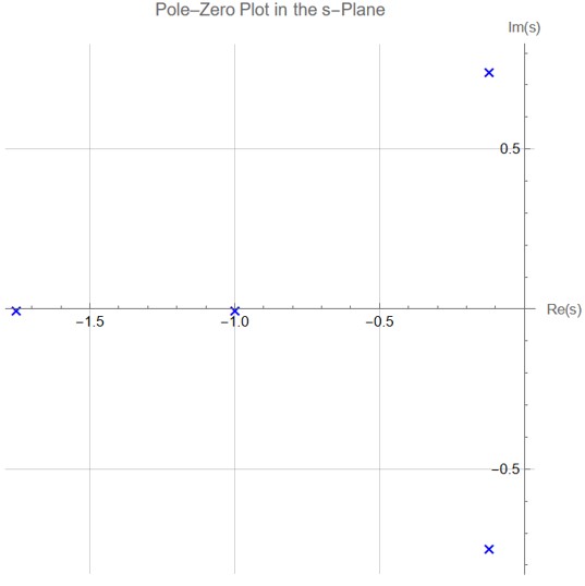
We can also confirm that this system is stable by plotting the poles as well. The figure confirms that all poles lie in the left half-plane.
This is our first tool to use for control design!
Controller Influence on Closed-Loop Poles and Stability
When designing a feedback control system, the dynamic behavior of the system is ultimately governed by the closed-loop transfer function, not the open-loop plant alone. This closed-loop behavior depends critically on the controller \( C(s) \), which appears directly in the closed-loop transfer function.

Given a plant \( P(s) \) and a controller \( C(s) \), the closed-loop transfer function with unity feedback can be calculated as follows:
\[
G(s) = \frac{Y(s)}{R(s)}
\]
where we know that in this system we can define the following relationships:
\[
C(s) = \frac{U(s)}{E(s)}, \quad
E(s) = R(s) - Y(s), \quad
P(s) = \frac{Y(s)}{U(s)}
\]
Now we can rearrange:
\[
U(s) = C(s)[R(s) - Y(s)] \Rightarrow Y(s) = P(s)C(s)[R(s) - Y(s)]
\]
Solve for \( Y(s) \):
\[
Y(s) + P(s)C(s)Y(s) = P(s)C(s)R(s) \Rightarrow
Y(s)[1 + P(s)C(s)] = P(s)C(s)R(s)
\]
Closed-loop transfer function:
\[
G(s) = \frac{Y(s)}{R(s)} = \frac{C(s)P(s)}{1 + C(s)P(s)}
\]
The poles of this system are the roots of the denominator:
\[
1 + C(s)P(s) = 0
\]
This is known as the characteristic equation of the closed-loop system. Its roots determine the stability and transient performance of the system. Importantly, these poles are directly influenced by the choice of controller \( C(s) \). This means we can shift the poles—and therefore the behavior—of the system by changing \( C(s) \).
Using Feedback to Stabilize an Unstable System
Suppose the open-loop system (plant) is unstable; that is, it has one or more poles in the right half of the \( s \)-plane. Using appropriate feedback, we can relocate these poles to the left half-plane (LHP), thereby stabilizing the system. This is one of the most powerful features of feedback control.
To illustrate this idea, consider a simple case where the controller is a constant gain:
\[
C(s) = K
\]
Then the closed-loop transfer function becomes:
\[
G_{\text{cl}}(s) = \frac{K P(s)}{1 + K P(s)}
\]
Let’s assume the plant is a first-order unstable system:
\[
P(s) = \frac{1}{s - a}, \quad \text{with } a > 0
\]
This system has an open-loop pole at \( s = a \), which lies in the right half-plane, so it is clearly unstable.
The closed-loop transfer function becomes:
\[
G_{\text{cl}}(s) = \frac{K}{s - a + K}
\]
The pole of the closed-loop system is at:
\[
s = a - K
\]
Now observe that:
- If \( K < a \), the pole remains in the right half-plane: the system is still unstable.
- If \( K = a \), the pole is at the origin: the system is marginally stable.
- If \( K > a \), the pole moves to the left half-plane: the system becomes stable.
This demonstrates that we can use the feedback gain \( K \) to shift the pole location and change an unstable system into a stable one.
Worked Example: Stability via Routh-Hurwitz
We are given a closed-loop transfer function of the form:
\[
G_{\text{cl}}(s) = \frac{(s + 1)k}{s^3 + 5s^2 + (k - 6)s + k}
\]
The denominator of the transfer function is the characteristic polynomial:
\[
P(s) = s^3 + 5s^2 + (k - 6)s + k
\]
We will determine the range of values of \( k \) that ensure the system is stable. This means all roots of \( P(s) \) must lie in the left-half of the \( s \)-plane, which is guaranteed if all the entries in the first column of the Routh-Hurwitz table are positive.
Step 1: Construct the Routh Table
\[
\begin{array}{c|cc}
s^3 & 1 & k - 6 \\
s^2 & 5 & k \\
s^1 & \frac{5(k - 6) - 1 \cdot k}{5} = \frac{5k - 30 - k}{5} = \frac{4k - 30}{5} & 0 \\
s^0 & k & 0
\end{array}
\]
Step 2: Routh-Hurwitz Stability Conditions
For stability, all entries in the first column must be positive:
- \( 1 > 0 \) — always true
- \( 5 > 0 \) — always true
- \( \frac{4k - 30}{5} > 0 \Rightarrow 4k - 30 > 0 \Rightarrow \boxed{k > 7.5} \)
- \( k > 0 \)
Thus, the system is stable when:
\[
\boxed{k > 7.5}
\]
This guarantees all the first-column entries of the Routh table are strictly positive, which implies the system is stable.

General Implications for Control Design
In practice, the controller \( C(s) \) may be more complex than a simple gain—it could include proportional-integral-derivative (PID) terms, lead/lag compensation, or state feedback. Regardless, the controller enters the closed-loop characteristic equation through the term \( 1 + C(s)P(s) \), and thus:
- All control objectives—such as stability, settling time, overshoot, and steady-state error—depend on the roots of this equation.
- Controller design is fundamentally about shaping the closed-loop pole locations to achieve desired performance.
- Even when the plant has undesirable dynamics (e.g., slow response, high overshoot, or instability), feedback can dramatically alter system behavior.
Caution: Feedback Can Also Destabilize a Stable System
While feedback can be used to stabilize an unstable system, the reverse is also true. Poorly designed feedback can move poles into the right half-plane and make a stable system unstable. For example, selecting a gain \( K \) that is too large can push a lightly damped complex-conjugate pair of poles into the unstable region, resulting in oscillations or runaway growth.
Thus, we must always verify closed-loop stability using:
- Analytical pole computation
- Routh-Hurwitz stability test
- Root locus or Nyquist criteria
Feedback Structure and Controller Design
In a unity feedback control system, the goal is for the output \( y(t) \) to track the reference \( r(t) \) in the presence of:
- Disturbance \( w(t) \): an external signal acting on the plant
- Sensor noise \( v(t) \): affecting the measured output

The key relationships:
\( e(t) = r(t) - y(t), \quad u(t) = C(s)e(t) \)
Control Design Objectives
1. Stability: All internal signals must remain bounded for all bounded inputs.
2. Tracking: Output \( y(t) \) should follow reference \( r(t) \) as \( t \to \infty \), assuming \( w(t) = v(t) = 0 \).
3. Disturbance Rejection: Output should stay close to \( r(t) \) even if \( w(t) \ne 0 \).
4. Control Effort Minimization: Minimize \( u(t) \) to prevent actuator saturation or damage.
Controller Gain Trade-offs
Let:
\( C(s) = K, \quad P(s) = \frac{1}{s + a} \)
Then:
\( T(s) = \frac{K}{s + a + K} \Rightarrow \) Pole shifts left with increasing \( K \)
Benefits of large \( K \):
- Reduced steady-state error
- Faster response (shorter \( t_s \))
- Improved tracking
Risks of large \( K \):
- Excessive control effort
- Potential actuator limitations
- Risk of destabilizing the system if the plant has lightly damped or unstable modes
Block Diagram Algebra for Closed-Loop Systems
For unity feedback, the closed-loop transfer function from reference \( r(t) \) to output \( y(t) \) is:
\[
\frac{Y(s)}{R(s)} = \frac{C(s)P(s)}{1 + C(s)P(s)}
\]
We can also calculate other relevant transfer functions:
\[
\frac{Y(s)}{R(s)} = \frac{C(s)P(s)}{1 + C(s)P(s)} \quad \text{(tracking)}
\]
\[
\frac{E(s)}{R(s)} = \frac{1}{1 + C(s)P(s)} \quad \text{(tracking error)}
\]
\[
\frac{E(s)}{W(s)} = \frac{-P(s)}{1 + C(s)P(s)} \quad \text{(regulation)}
\]
\[
\frac{U(s)}{R(s)} = \frac{C(s)}{1 + C(s)P(s)} \quad \text{(control effort)}
\]
The denominator \( 1 + C(s)P(s) \) is shared across all closed-loop transfer functions, and its roots determine closed-loop stability.
We can also use this very helpful table to determine the numerator for transfer functions here but remember that this is only for unity feedback.

Once the feedback loop is closed, the system no longer behaves like the open-loop plant. Instead, its dynamics are governed entirely by the <strong>closed-loop transfer function</strong>, which depends directly on the controller \( C(s) \).
Remember, to guarantee that the closed-loop system is stable, <strong>all poles of the transfer function must lie in the left half of the complex \( s \)-plane</strong>. For real poles, this means each must satisfy \( \text{Re}(s_i) < 0 \).
Interpretation of These Transfer Functions
Stability: We want all real values of the poles to be less than zero and to satisfy our previous stability criteria.
Tracking: To achieve good tracking, we want the output \( y(t) \) to follow the reference \( r(t) \) closely. This implies the tracking error \( e(t) = r(t) - y(t) \) should be small. From:
\[
\frac{E(s)}{R(s)} = \frac{1}{1 + C(s)P(s)}
\]
we see that increasing the magnitude of \( C(s) \) (controller gain) reduces this quantity, leading to better tracking performance.
Regulation: Similarly, to reject disturbances \( w(t) \), we require:
\[
\frac{E(s)}{W(s)} = \frac{-P(s)}{1 + C(s)P(s)}
\]
to be small in magnitude. Again, a larger \( C(s) \) suppresses the impact of disturbances on the error. In this case, we say the controller has high authority, meaning it dominates the behavior of the system.
Control Effort: However, increasing controller gain also increases the required actuation. From:
\[
\frac{U(s)}{R(s)} = \frac{C(s)}{1 + C(s)P(s)}
\]
we observe that if \( C(s) \) is too large, the control effort \( u(t) \) may become excessive. This could lead to actuator saturation, overheating, or inefficiency, especially if \( P(s) \) has limited bandwidth or sensitivity.
Trade-Off Between Tracking and Effort
There is a fundamental trade-off in feedback control:
Larger \( C(s) \): better tracking, better disturbance rejection, but more control effort
Smaller \( C(s) \): less effort, but poorer performance
Example: Gain Controller
Consider a proportional controller: \( C(s) = K \), and suppose the plant is:
\[
P(s) = \frac{1}{s - 2}
\]
This plant is unstable (it has a pole at \( s = 2 \) in the right-half plane).
The closed-loop transfer function becomes:
\[
G_{\text{cl}}(s) = \frac{K}{s - 2 + K}
\]
The closed-loop pole is located at:
\[
s = 2 - K
\]
Analysis:
If \( K < 2 \), the pole remains in the RHP \( \Rightarrow \) unstable
If \( K = 2 \), the pole is at the origin \( \Rightarrow \) marginally stable
If \( K > 2 \), the pole moves to the LHP \( \Rightarrow \) system becomes stable
Thus, by selecting \( K > 2 \), feedback control stabilizes the system.
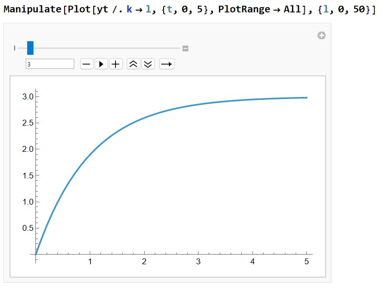
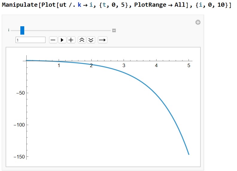
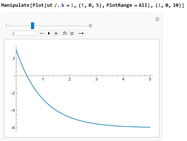
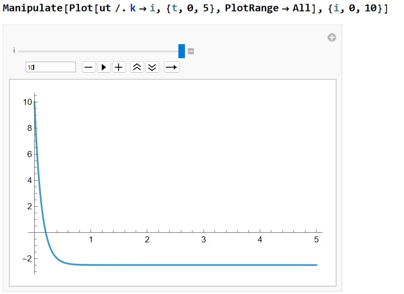
Assume a unit step input \( r(t) = 1 \Rightarrow R(s) = \frac{1}{s} \). Then the output becomes:
\[
Y(s) = G(s) \cdot R(s) = \frac{K}{(s - 2 + K)s}
\]
We can see the system response here from unstable, to stable, to improved performance as \( K \) increases.


We define the control effort in the Laplace domain as:
\[
U(s) = C(s) \cdot E(s) = C(s) \cdot (R(s) - Y(s))
\]
Alternatively, we can derive \( U(s) \) directly as:
\[
U(s) = \frac{C(s)}{1 + C(s)P(s)} \cdot R(s)
= \frac{K}{1 + \frac{K}{s - 2}} \cdot \frac{1}{s}
= \frac{K(s - 2)}{(s + (K - 2))s}
\]
Thus:
\[
U(s) = \frac{K(s - 2)}{s(s + (K - 2))}
\]
We can see the system response for an unstable, stable, and controller response for larger \( K \) here.
Trade-Off and Risk of Instability
While increasing \( K \) improves tracking and speeds up convergence, it also:
Increases required actuation \( u(t) \)
May exceed actuator limits (saturation, overheating)
Can destabilize the system if \( P(s) \) has fragile dynamics
Even though we started with an unstable plant, we can stabilize it with \( K > 2 \). However, this comes at the cost of potentially excessive control effort.
If we attempt to apply a similar strategy to a different plant (e.g., a stable but lightly damped one), increasing \( K \) without analysis may introduce instability through:
Poorly located poles
Reduced phase margin
Interaction with delays or non-minimum phase elements
Example: Feedback Can Destabilize a Stable Plant
In this example, we explore how a poorly chosen controller can destabilize an otherwise stable system. Let:
\[
P(s) = \frac{2}{s + 1}, \quad C(s) = \frac{s - k}{s + 2}
\]
This represents a stable first-order plant (pole at \( s = -1 \)) and a controller that introduces both a pole at \( s = -2 \) and a zero at \( s = k \), where \( k \in \mathbb{R} \) is a tunable parameter.
Closed-Loop Transfer Function
Under unity feedback, the closed-loop transfer function is:
\[
G_{\text{cl}}(s) = \frac{C(s) P(s)}{1 + C(s) P(s)}
= \frac{\left(\frac{s - k}{s + 2}\right) \cdot \left(\frac{2}{s + 1}\right)}{1 + \left(\frac{s - k}{s + 2}\right) \cdot \left(\frac{2}{s + 1}\right)}
\]
Multiply numerator and denominator:
\[
G_{\text{cl}}(s) = \frac{2(s - k)}{(s + 2)(s + 1) + 2(s - k)}
\]
Now simplify the denominator:
\[
(s + 2)(s + 1) = s^2 + 3s + 2
\]
\[
2(s - k) = 2s - 2k
\]
\[
\Rightarrow \text{Denominator: } s^2 + 3s + 2 + 2s - 2k = s^2 + 5s + 2 - 2k
\]
So the closed-loop transfer function becomes:
\[
G_{\text{cl}}(s) = \frac{2(s - k)}{s^2 + 5s + 2 - 2k}
\]
<h5>Characteristic Equation</h5>
To analyze stability, we examine the denominator:
\[
s^2 + 5s + (2 - 2k) = 0
\]
Let us denote the characteristic polynomial:
\[
P(s) = s^2 + 5s + (2 - 2k)
\]
This is a second-order polynomial. To ensure stability, both roots must lie in the left-half complex plane. This happens if and only if:
All coefficients are positive
The roots have negative real parts
Condition 1: Positive Coefficients
We already have:
\[
\text{Coefficient of } s^2 = 1 > 0, \quad \text{Coefficient of } s = 5 > 0
\]
So we require:
\[
2 - 2k > 0 \Rightarrow k < 1
\]
Condition 2: Discriminant
The roots are given by:
\[
s = \frac{-5 \pm \sqrt{25 - 4(2 - 2k)}}{2}
= \frac{-5 \pm \sqrt{25 - 8 + 8k}}{2}
= \frac{-5 \pm \sqrt{17 + 8k}}{2}
\]
This is always real for \( k \geq -\frac{17}{8} \), but we care only about whether both roots are in the left half-plane.
From the quadratic formula, regardless of whether the roots are real or complex, the real part of both roots is always:
\[
\frac{-5}{2} < 0
\]
So stability in this case is entirely determined by the constant term:
\[
\boxed{k < 1}
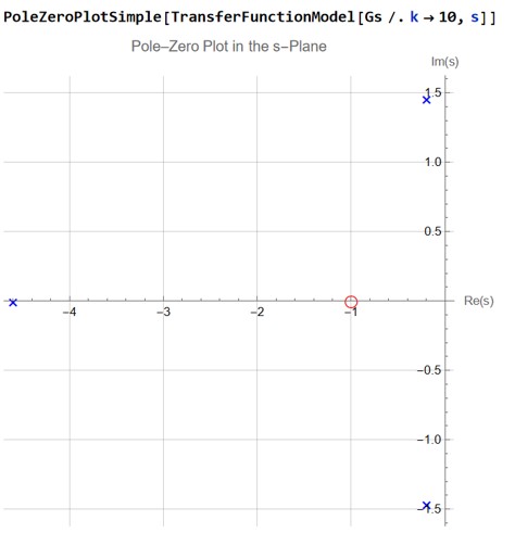
\]
We can see the poles here:
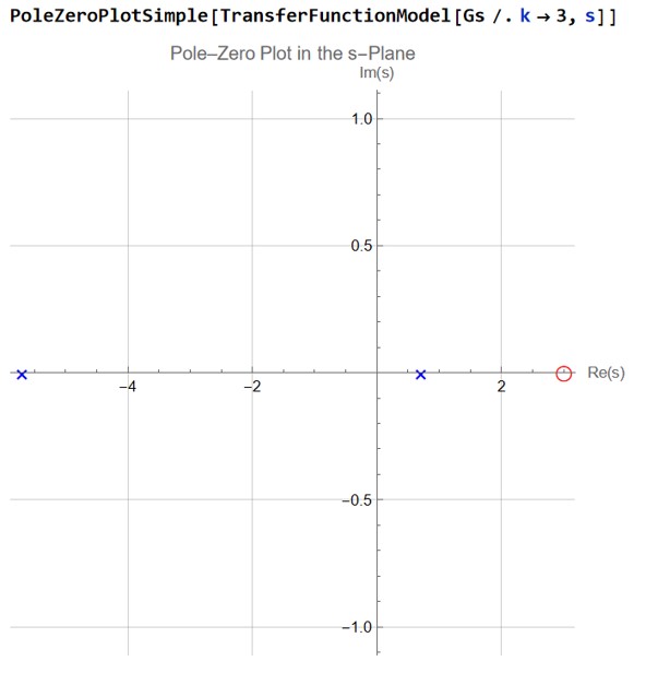

Conclusion
The closed-loop system becomes unstable when the controller zero is placed to the right of \( s = 1 \). This illustrates an important concept:
Even though the plant \( P(s) = \frac{2}{s + 1} \) is stable,
and the controller has stable dynamics \( C(s) = \frac{s - k}{s + 2} \),
the interaction between the controller and plant introduces a pole-zero interplay that can destabilize the system.
Key Insight
Stability is not guaranteed just because individual components are stable. The location of the controller zero (at \( s = k \)) can destabilize the system if it disrupts the structure of the closed-loop poles.
Design Rule: Avoid placing controller zeros too far to the right, especially when they affect low-order or lightly damped systems.
This example illustrates a central principle of control design:
Feedback allows us to change pole locations and stabilize unstable systems.
Increased controller gain improves performance (faster \( y(t) \), smaller \( e(t) \)).
However, excessive gain increases \( u(t) \) and may destabilize the system.
We must balance performance, control effort, and robustness.
This is why pole placement, root locus, and frequency response tools are essential for rigorous controller design.
Feedback is powerful but can be dangerous if misapplied. For example, if the plant is already stable, adding a high-gain controller without considering phase margin or bandwidth limitations can introduce unwanted dynamics (e.g., unstable pole-zero cancellations, delayed phase lag). Therefore, control design must always verify:
Stability (pole locations in LHP)
Performance (settling time, overshoot)
Feasibility (bounded control effort)
Feedback control enables designers to systematically modify system dynamics, improve performance, and reject disturbances. However, this power must be exercised with care. Poorly tuned controllers may consume excessive energy or destabilize the system. Control design is therefore a process of negotiation between performance, robustness, and practical constraints.
In future topics, we will explore controller structures such as PID, root locus design, and frequency-domain techniques (Bode, Nyquist), all of which build on this foundation of time-domain performance, stability, and block diagram relationships.