Chapter 13: Frequency Response, Nyquist Stability Criterion, and Bode Plots

Sinusoidal Steady-State Behavior

For any linear time-invariant (LTI) system, a sinusoidal input of frequency \( \omega \) will produce a sinusoidal output of the same frequency, but scaled in amplitude and phase-shifted. Mathematically:

\[
u(t) = A \cos(\omega t) \quad \Rightarrow \quad y(t) = |G(j\omega)| A \cos(\omega t + \angle G(j\omega))
\]

This output structure allows us to define the frequency response function:

\[
\boxed{G(j\omega) = |G(j\omega)| e^{j \angle G(j\omega)}}
\]

Here:

- \( |G(j\omega)| \): gain or magnitude response
- \( \angle G(j\omega) \): phase response (typically in degrees or radians)

This substitution arises from evaluating the Laplace-domain transfer function at \( s = j\omega \), transforming the problem into an algebraic computation.

Physical Insight: Mass-on-Sheet Example

Imagine a small coin (mass) resting on a sheet of paper that moves sinusoidally side to side.

- At low frequencies: the coin moves nearly identically with the paper. The system tracks the input well.
\[
|G(j\omega)| \approx 1, \quad \angle G(j\omega) \approx 0^\circ
\]
- At high frequencies: inertia dominates. The coin barely moves while the paper vibrates beneath it.
\[
|G(j\omega)| \ll 1, \quad \angle G(j\omega) \to -90^\circ \text{ (or more)}
\]

This setup shows that the frequency response captures not only gain attenuation but also the phase lag introduced by system dynamics.

Frequency Response from Transfer Functions

Given a transfer function:

\[
G(s) = \frac{N(s)}{D(s)}
\]

its frequency response is:

\[
G(j\omega) = \frac{N(j\omega)}{D(j\omega)} = \frac{|N(j\omega)| e^{j \angle N(j\omega)}}{|D(j\omega)| e^{j \angle D(j\omega)}}
= |G(j\omega)| e^{j \angle G(j\omega)}
\]

In this form, we can easily compute the gain and phase at each frequency. This is the basis for constructing Bode and Nyquist plots.

Bode Plots

The Bode plot consists of two separate plots versus \( \log_{10}(\omega) \):

1. Magnitude Plot:
\[
20 \log_{10} |G(j\omega)|
\]

2. Phase Plot:
\[
\angle G(j\omega) \quad (\text{in degrees})
\]

Each elementary component of \( G(s) \)—poles, zeros, gain, integrators—has a well-known log-magnitude and phase contribution. The product of transfer function terms becomes the sum in log scale:

\[
\log_{10}(ab) = \log_{10}(a) + \log_{10}(b)
\]

This is why Bode plots use logarithmic magnitude and linear phase: they simplify system composition to visual addition.

Seven Elementary Transfer Functions

All rational transfer functions can be constructed from combinations of these elementary blocks:

1. Constant gain \( K \)
2. Pure integrator: \( \frac{1}{s} \)
3. First-order pole: \( \frac{1}{s + a} \)
4. First-order zero: \( s + a \)
5. Second-order term:
\[
\frac{\omega_n^2}{s^2 + 2\zeta \omega_n s + \omega_n^2}
\]
6. Differentiator: \( s \)
7. Time delay: \( e^{-sT} \) (phase-only effect)

Bode plots for complex systems are built by superposing the Bode plots of these building blocks.

Nyquist Plot

The Nyquist plot is a parametric plot of \( G(j\omega) \) in the complex plane as \( \omega \in [0, \infty) \). It displays the real and imaginary parts of the frequency response:

\[
G(j\omega) = \text{Re}(\omega) + j \cdot \text{Im}(\omega)
\]

This plot encodes both gain and phase simultaneously and plays a central role in stability analysis.

Construction methods:

- Method 1: Sketch from Bode plot
- Sweep frequency from \( \omega = 0^+ \to \infty \)
- Record gain and phase at sample points
- Mirror the plot across the real axis for \( \omega < 0 \)
- Indicate arrows (direction of increasing frequency)

- Method 2: Parametric plot of \( G(j\omega) \)
\[
\omega \mapsto \left( \text{Re}[G(j\omega)], \text{Im}[G(j\omega)] \right)
\]
This method is often implemented numerically or using symbolic tools like Mathematica.

Worked Bode and Nyquist Plot Examples

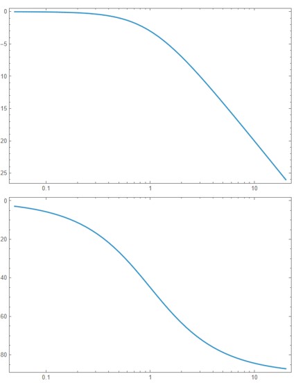
Example 1: First-Order Low-Pass Filter

Let:
\[
G(s) = \frac{1}{s + 1}
\]

Frequency Response:
\[
G(j\omega) = \frac{1}{j\omega + 1} = \frac{1}{\sqrt{\omega^2 + 1}} \angle -\tan^{-1}(\omega)
\]

Bode Plot:
- Magnitude: \( 20 \log_{10} \left( \frac{1}{\sqrt{\omega^2 + 1}} \right) \)
- Phase: \( -\tan^{-1}(\omega) \)
- At \( \omega = 1 \): -3 dB, phase = -45°

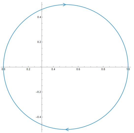
Nyquist Plot:
- Starts at \( G(0) = 1 \)
- Arcs toward the origin in the fourth quadrant
- Never crosses or encircles -1

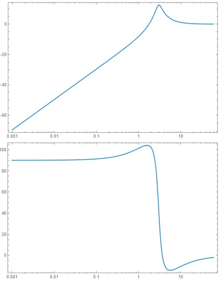
Example 2: Second-Order System with Resonance

Let:
\[
G(s) = \frac{s(s + 3)}{s^2 + s + 9}
\]

Frequency Response:
\[
G(j\omega) = \frac{j\omega(j\omega + 3)}{(j\omega)^2 + j\omega + 9}
\]

Use symbolic tools or software to evaluate magnitude and phase across frequencies.

Key Observations:
- Resonant peak near \( \omega = 3 \)
- Magnitude plot shows a dip followed by a peak
- Phase starts near \( +90^\circ \), decreases, and drops toward \( -90^\circ \)

Nyquist Plot:
- Begins at origin
- Swirls outward due to the numerator zero at \( s = -3 \)
- Shows high-frequency behavior consistent with a second-order system

Example 3: Lead Controller Behavior

Let:
\[
G(s) = \frac{s + 1}{s + 10}
\]

Frequency Response:
\[
G(j\omega) = \frac{j\omega + 1}{j\omega + 10}
\]

Magnitude:
\[
|G(j\omega)| = \frac{\sqrt{\omega^2 + 1}}{\sqrt{\omega^2 + 100}} \Rightarrow \text{High-frequency gain} \to 1/10 = -20\,\text{dB}
\]

Phase:
\[
\angle G(j\omega) = \tan^{-1}(\omega) - \tan^{-1}(\omega/10) \Rightarrow \text{Positive phase bump — typical of lead compensation}
\]

Nyquist Plot:
- Arc in the right-half plane (phase lead)
- Ends closer to the real axis
- Useful for bending root locus toward the left

Nyquist Stability Criterion

The Nyquist criterion is a frequency-domain test that links the stability of a closed-loop system to the open-loop transfer function.

Let:
\[
L(s) = C(s)P(s) \quad \Rightarrow \quad T(s) = \frac{L(s)}{1 + L(s)}
\]

The closed-loop poles are the roots of \( 1 + L(s) = 0 \).

Nyquist Criterion:
\[
Z = P - N
\]

Where:
- \( Z \): number of closed-loop poles in the right-half plane (unstable)
- \( P \): number of open-loop poles in the RHP
- \( N \): number of counter-clockwise encirclements of the point \( -1 + j0 \) by the Nyquist plot of \( L(j\omega) \)

Interpretation:
- For stability, we want \( Z = 0 \Rightarrow N = P \)
- If \( L(s) \) has no RHP poles (\( P = 0 \)), then stability requires no encirclements of \( -1 \)

This criterion is a consequence of the argument principle in complex analysis, mapping the number of encirclements of a critical point to the number of zeros of a function inside a contour.

Important Considerations: Poles at the Origin

When \( L(s) \) has poles on the imaginary axis (e.g., integrators at \( s = 0 \)), the Nyquist contour must be indented to avoid singularities. In practice:

- The contour detours around the origin in the complex plane
- We analyze \( \lim_{\omega \to 0^+} L(j\omega) \)
- The mapping of the contour near the origin contributes a large arc in the complex plane

If the pole at the origin is stable (i.e., not causing exponential growth), then it does not increase \( P \), but it does affect the Nyquist plot's shape and must be handled carefully.

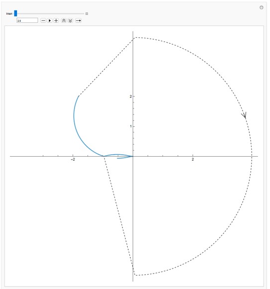
Worked Example 1: Nyquist Stability Analysis

Let:
\[
L(s) = \frac{k(s + 2)}{s(s^2 + s + 3)}
\]

Step 1: Open-loop Pole and Zero Locations
- One integrator pole at \( s = 0 \)
- Two complex poles from \( s^2 + s + 3 \):
\[
s = \frac{-1 \pm \sqrt{1 - 12}}{2} = \frac{-1 \pm j\sqrt{11}}{2}
\]
- One zero at \( s = -2 \)

This means:
\[
P = 0 \quad \text{(no open-loop RHP poles)}
\]

Step 2: Nyquist Stability Criterion
We check:
\[
Z = P - N \quad \Rightarrow \quad Z = -N
\]
To ensure stability, we want \( Z = 0 \Rightarrow N = 0 \), i.e., no encirclements of \( -1 \).

Step 3: Find Critical Frequency
We solve numerically for the frequency \( \omega_{\text{crit}} \) where:
\[
\angle L(j\omega) = -180^\circ
\]
This occurs at:
\[
\boxed{\omega_{\text{crit}} \approx 2.44 \ \text{rad/s}}
\]

Step 4: Compute Gain at That Frequency
Evaluate:
\[
|L(j\omega_{\text{crit}})| \approx 0.337
\quad \Rightarrow \quad
\boxed{k_{\text{crit}} \approx \frac{1}{0.337} = 2.97}
\]

Conclusion:
- For stability: \( \boxed{k < 2.97} \)
- For \( k > 2.97 \), the Nyquist plot encircles \( -1 \Rightarrow Z = 1 \Rightarrow \) closed-loop unstable
- For \( k = 2.97 \), the system is marginally stable

Worked Example 2: Nyquist Analysis with RHP Pole

Let:
\[
L(s) = \frac{k(s + 1)}{s - 2}
\]

Step 1: Pole-Zero Structure
- One zero at \( s = -1 \)
- One pole at \( s = +2 \quad \Rightarrow \boxed{P = 1} \)

This system has an <b>open-loop unstable pole</b> at \( s = +2 \), so we must ensure:
\[
Z = P - N = 1 - N \Rightarrow \boxed{N = 1} \text{ (for closed-loop stability)}
\]

In other words, we require the Nyquist plot of \( L(j\omega) \) to make <b>one counterclockwise encirclement of \( -1 \)</b> for the closed-loop system to be stable.

Step 2: Frequency Response

\[
L(j\omega) = \frac{k(j\omega + 1)}{j\omega - 2}
\]

Compute the magnitude and phase:
\[
|L(j\omega)| = \frac{k \cdot \sqrt{\omega^2 + 1}}{\sqrt{\omega^2 + 4}}
\]
\[
\angle L(j\omega) = \tan^{-1}(\omega) - \pi - \tan^{-1}\left( \frac{\omega}{-2} \right)
\]

Step 3: Critical Frequency for Instability

At \( \omega = 0 \), the phase is exactly \( -180^\circ \), and:
\[
L(j0) = \frac{k(1)}{-2} = -\frac{k}{2}
\Rightarrow |L(j0)| = \frac{k}{2}
\]

Set \( |L(j0)| = 1 \Rightarrow \boxed{k_{\text{crit}} = 2} \)

Step 4: Interpretation

Since the system has a RHP pole at \( s = 2 \), the Nyquist criterion requires:
\[
\boxed{\text{One CCW encirclement of } -1}
\]

That means:
- For \( k < 2 \), the Nyquist plot does <b>not</b> encircle \( -1 \) \( \Rightarrow \) closed-loop unstable
- For \( k = 2 \), the Nyquist plot <b>touches</b> \( -1 \) \( \Rightarrow \) marginally stable
- For \( k > 2 \), the plot <b>encircles</b> \( -1 \) once \( \Rightarrow \) closed-loop stable

Conclusion:
- Open-loop instability (\( P = 1 \)) requires one CCW encirclement of \( -1 \)
- Closed-loop stability is possible, but only if gain is tuned: \( \boxed{k > 2} \)
- Nyquist and Bode gain/phase margin analysis helps determine safe bounds on \( k \)

Conclusion

- Root locus and frequency response tools like Nyquist plots and Bode plots are critical to understanding system stability and performance.
- Bode plots provide insight into gain and phase margins, bandwidth, and resonance behavior.
- Nyquist plots visualize the response in the complex plane and help determine closed-loop stability even for systems with open-loop unstable poles.
- Nyquist stability criterion states:
\[
Z = P - N
\]
where:
- \( Z \): number of unstable closed-loop poles
- \( P \): number of open-loop poles in the right-half plane
- \( N \): number of counter-clockwise encirclements of \( -1 \) by the Nyquist plot

- For a system to be stable, we want \( Z = 0 \), which implies:
- If \( P = 0 \), then \( N = 0 \) (no encirclements of -1)
- If \( P = 1 \), then \( N = 1 \) (one counter-clockwise encirclement of -1)

Design Guidelines

- Use Bode plots to evaluate gain and phase margins.
- Use Nyquist plots to assess closed-loop stability and validate against the Nyquist criterion.
- Tune controller gain to achieve desired margins while ensuring system stability:
- Avoid crossing the -1 point in the Nyquist plot without satisfying the Nyquist condition.
- Use frequency response plots to choose gains that avoid excessive phase lag or resonant peaking.