Chapter 4: Fourier Analysis and Continuous Fourier Transforms

Fourier Analysis Applications

Before we get into talking about Fourier Analysis and getting in the weeds of continuous fourier transforms, discrete, spectrum analysis, signal aliasing, and spectral leakage let's take a step back and see why this analysis is useful or helpful.

Fourier analysis is a critical tool common to engineers and experimentalists, it is extremely ubiquitous and interdisciplinary. Fourier Analysis generally involves measuring some signal that varies as a function of time, one then performs a Fourier transform which allows one to examine how that signal varies in the frequency space or domain instead of the time domain. Because we know that time and frequency are inversely related you are essentially looking at a signal in one space, whether that be time, distance, etc and then you transform the signal to examine the behavior in some reciprocal space or domain.

Time to Frequency Space or Reciprocal Space

I understand that sounds very very confusing so let's look at a couple of practical applications of Fourier Analysis. One of the most common types of Fourier Analysis involves looking at a signal whether it be electrical, mechanical, optical, etc. and performing a Fourier Transform to look at the signal in frequency space via a Fourier Spectrum graph, much more on this later. We can then examine these Frequency Spectrum curves which show the amplitude of our harmonic coefficients as a function of frequency and we can identify many things about the signal we are measuring including:

- Fundamental or Lowest Frequency
- Maximum Frequency
- Dominant Frequency

These are critical parameters that will allows us to make decisions about the design of our application or experimental apparatus. As you can see in the example above these two signals are distinct in terms of frequencies and we see in the resultant Frequency Spectrum curves there are also distinct changes in these curves as well.

ECG Measurements

An electrocardiogram (ECG) is a truly amazing measurement as we are effectively seeing in the curve above the bio-potential, the voltage generated from heart cells. Now typically cells can produce a potential of around 100mV. As you can see on the curve above we are measuring around 1mV but this is amazing!! Through all the tissue, blood, fluids, collagen, bone, etc we are able to measure the potential of a heart cell with electrodes placed on our skin. Really amazing! We can then take this signal and perform a Fourier transform and identify anomalous frequencies to make a diagnosis for irregular heartbeats and other issues.

We can also see some high and low frequency noise in our signal and who can blame us we are measuring the voltage a heart cell at distances on the meter length scale away. The beauty of Fourier analysis is we can identify the high and low frequency noise typically expected for ECG measurements and then we can build high and low pass frequency filters that filter out this noise and improve our original signal of interest.

Differences in Musical Instruments

We can also utilize Fourier Transforms to distinguish between the same note being played by different instruments. We can record the sound being played and measure the voltage registered by the recording device and then perform a Fourier transform on the voltage vs time signal to convert to our Frequency Spectrum curve where the frequency is on the x-axis.

Distinguish Between Vocal Sounds, Ahh, Eee, Ooo

Fourier analysis can similarly be used to distinguish between vowel sounds. You must appreciate my effort in this course as I recorded myself saying these words over and over and looked very foolish indeed. However, I was able to acquire data as a function of time and voltage and performed my Fourier Analysis.

XRD Reciprocal Space and Bragg's Law

As I have stated many times, my background is in Materials Science and Engineering, and one of the most critical tools to analyze the structure of materials is via X-Ray Diffraction (XRD). In XRD, you shoot an incident beam of radiation — typically Cu\(_\alpha\) radiation — and that wavelength of radiation at certain angles, called Bragg Angles, will constructively interfere with planes of atoms.

We can then use simple trigonometric identities to calculate the interplanar distance \( d_{hkl} \) between these planes (or more generally any distance between periodic arrays of atoms), as described by Bragg's Law:

$$
n \lambda = 2d_{hkl} \sin(\theta)
\]

Where:
- \( n \) is a positive integer
- \( \lambda \) is the wavelength of the radiation, typically Cu\(_\alpha\), which is 1.56 Å

The XRD output is a graph of the intensity of the diffracted radiation as a function of \( 2\theta \). Now if we look at Bragg's Law, we can see that the distance \( d \) that we are trying to measure is inversely related to \( \theta \), so the graph of intensity vs. \( 2\theta \) is effectively a plot of intensity vs. **reciprocal space**, i.e., \( \frac{1}{d} \). This is very similar to what we have seen previously: a plot of inverse time space or frequency space.

We can use XRD to determine characteristic distances between or within polymer chains. Remember: XRD is looking for periodic distances within polymer structures, and we can only measure distances that exhibit some degree of order — either short-range or long-range.

We can see an example of this unique type of Fourier analysis by looking at a family of methacrylate polymers — specifically PMMA, PPMA, PEMA, and PBMA — which vary in the R length. In this case, the end group is a methyl, CH₃.

Now if we place these polymers within the XRD, we can obtain the following XRD curves:

As you can see, we observe multiple peaks in our XRD curves. A peak in the intensity correlates to when we obtain constructive interference. Thus, at that angle — or equivalently, at that inverse distance — there is some distance in the polymer that has some degree of long-range or short-range order.

You can also see that some of the peaks in the curve are conserved — i.e., the peaks at larger \( 2\theta \) values appear at essentially the same location. However, the peaks at low \( 2\theta \) angles appear to shift based on the polymer. This suggests there is some characteristic, repeated, periodic, or ordered structure/distance in the polymer chain.

The question then becomes: Why do some distances in the polymer chain change?

To understand this, we must look at the chemical structure of our methacrylate polymers.

We saw previously that the primary structural difference between our methacrylate polymers is the length of the pendant side chain, i.e., the number of CH₃ (R groups). From this schematic:

- Intra-chain distances will **not** change — these are fixed bond lengths (like the C–C bond ≈ 1.54 Å)
- Inter-segmental distances will **not** change
- Inter-chain and intra-segment distances **will** change as R increases

Now back to our XRD plots — which peaks correspond to which distances?

- Peaks at large \( 2\theta \): these correspond to **small** distances (like intra-chain), and they don’t shift — they are conserved
- Peaks at small \( 2\theta \): these correspond to **larger** distances (like inter-chain), and they do shift to lower angles as R increases

Why do peaks shift left with increasing R?

Because as R increases, inter-chain distances increase. So the associated angle \( \theta \) must decrease to satisfy Bragg’s Law (since \( \sin(\theta) \propto \frac{1}{d} \)), and thus \( 2\theta \) shifts left.

This is the power of Fourier Analysis again — XRD gives us a reciprocal-space view of periodic structures and allows us to infer real-space behavior through mathematical transformation.

Photo 51: Rosalind Franklin

Hopefully everyone has seen this image before. What is it? Don't read the caption.

This is Rosalind Franklin's Photo 51 — an XRD picture of a DNA fiber from a calf thymus — which was then analyzed by Watson and Crick who were later credited for the discovery of DNA. Rosalind Franklin was an amazing chemist and X-ray crystallographer; however, Watson and Crick knew about Fourier.

So when they saw this picture they could clearly make out this reciprocal space image and reconstruct the structure of DNA. Rosalind Franklin was not given credit for her contribution until after her death. She died at age 37 due to ovarian cancer — a tragic story, but again showing the importance of Fourier Analysis. History books would have been written completely differently.

Time Varying Measurements, Harmonic Functions, Cyclic and Circular Frequency:

We have previously discussed in Lecture 1 that all measurands will vary as a function of time and they can be static, dynamic, periodic, aperiodic, etc. The power and beauty of Fourier Transforms — as we will see soon — is that regardless of how the signal varies in time we will be able to analyze this using the framework of Fourier Analysis.

Now many of the signals that we will analyze will be periodic in nature and many of them will be harmonic functions. You have likely encountered many harmonic functions in your career as an engineer and hopefully have worked with sine and cosine functions. A function \( y(t) \) can be classified as harmonic if:

$$
\frac{\partial^2 y}{\partial t^2} = -c y(t)
\]

Where \( c \) is a constant.

Prove that both cosine and sine are harmonic functions. What about \( y(t) = x^2 \)?

These harmonic functions — and really all functions — can be treated over some period \( T \) as periodic. These functions will exhibit some frequency, and here we must distinguish:

- Circular Frequencies \( \omega \)
- Cyclic Frequencies \( f \)

Circular frequency is related to cyclic frequency as:

$$
\omega = 2\pi f
\]

Where \( \omega \) is in rad/s and \( f \) is in Hz. In this course we will always use cyclic frequency \( f \) in SI units. However, you may see \( \omega \) in problems or real-world systems, so be sure to convert when necessary.

Continuous Fourier Transforms: Calculating Harmonic Coefficients

Finally we are about to undertake the task of performing a Fourier Transform. Just a warning — the math will get a bit tricky here — but do not get lost in the math. Keep your high-level conceptual understanding that we developed by looking at the examples above.

So when we are analyzing a signal and we have the algebraic expression of our signal \( y(t) \), i.e., we know for example \( y(t) = \cos(t) \). We must transform this signal from time space \( t \) to reciprocal time space or frequency space \( f \). To do this we must calculate the harmonic coefficients of our Fourier Series, \( A_n \) and \( B_n \). These harmonic coefficient values at different integer values \( n \) will be critical to create our frequency spectrum. They will also allow us to represent any arbitrary signal \( y(t) \) as an infinite sum of sines and cosines when we represent our original signal \( y(t) \) as a Fourier Series.

That was a lot to take in — let's just focus for the moment on how to calculate our harmonic coefficients.

To calculate our harmonic coefficients we can perform the following analysis:

$$
A_n = \frac{\omega}{\pi} \int_0^{\frac{2\pi}{\omega}} y(t) \cos(\omega n t) \, dt \quad n = 0, 1, 2, \ldots
\]

$$
B_n = \frac{\omega}{\pi} \int_0^{\frac{2\pi}{\omega}} y(t) \sin(\omega n t) \, dt \quad n = 0, 1, 2, \ldots
\]

Where:
- \( A_n \), \( B_n \): harmonic coefficients
- \( y(t) \): your original signal
- \( n \): the order of the harmonic coefficient
- For example, if you are asked for the 3rd harmonic coefficient, compute \( A_3 \), \( B_3 \)

You will integrate your original signal with respect to time and keep \( n \) in your solution. Then you will calculate the harmonic coefficients for increasing values of \( n \) until you sufficiently represent the signal of interest.

However, as you can see in the expression above, we have an issue — we do not want to work with our function in terms of \( \omega \); we want to work with \( f \). So we substitute using:

$$
\omega = 2\pi f
\]

Additionally, we typically analyze a function or signal for a finite period of time \( T \). The lowest (fundamental) frequency of any signal is:

$$
f_{\text{fundamental}} = \Delta f = \frac{1}{T}
\]

So then:

$$
\omega = \frac{2\pi}{T}
\]

Plugging this into the harmonic coefficient expressions gives the form we will use in this course:

$$
A_n = \frac{2}{T} \int_0^T y(t) \cos\left( \frac{2\pi n t}{T} \right) dt \quad n = 0, 1, 2, \ldots
\]

$$
B_n = \frac{2}{T} \int_0^T y(t) \sin\left( \frac{2\pi n t}{T} \right) dt \quad n = 0, 1, 2, \ldots
\]

Once we have our harmonic coefficients, we calculate their magnitudes:

$$
C_n = \sqrt{A_n^2 + B_n^2}
\]

This value \( C_n \) is what we will plot as the y-axis on the Frequency Spectrum, and the x-axis will be the corresponding frequency values — which are integer multiples of the fundamental frequency \( f = \frac{1}{T} \).

That is a lot of information to take in, so let's do an example to make this clear…

Harmonic Coefficients, Frequency Spectrum, Dominant Frequency, Maximum Frequency

It's Hip to Be Square

We have the following curve of displacement and time. Calculate the Frequency Spectrum and the Fourier Series for this curve.

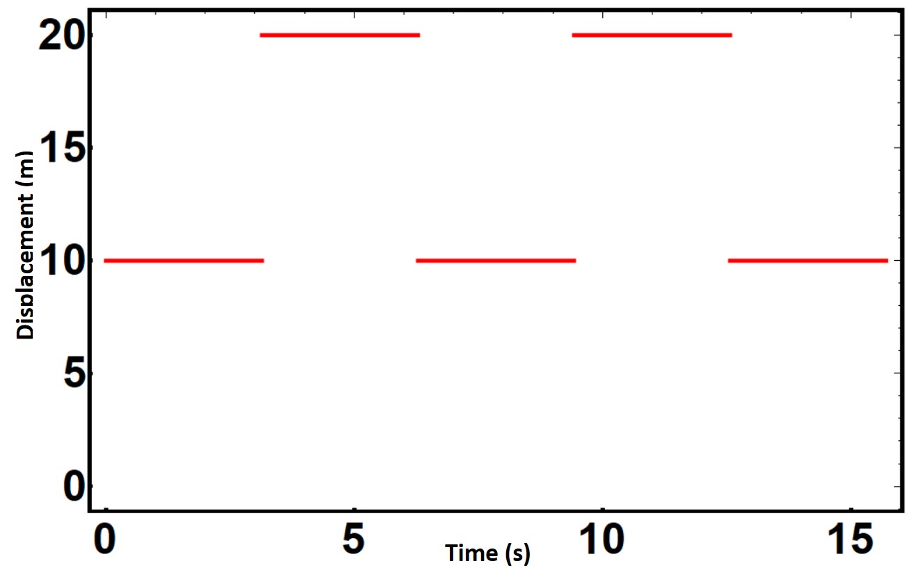
When looking at this curve it is a square wave, hence the Huey Lewis reference. Thus we can describe piece-wise the algebraic form of this function. Specifically we know that:

$$
y_{1}(t) = 10 \quad 0 < t < \pi \\
y_{2}(t) = 20 \quad \pi < t < 2\pi
\]

Now that we have our \( y(t) \), we can calculate our harmonic coefficients \( A_n \) and \( B_n \). So again we have:

$$
A_n = \frac{2}{T} \int_0^T y(t) \cos\left(\frac{2\pi n t}{T}\right) dt \quad n = 0, 1, 2, \ldots \\
B_n = \frac{2}{T} \int_0^T y(t) \sin\left(\frac{2\pi n t}{T}\right) dt \quad n = 0, 1, 2, \ldots
\]

Where:
- \( T \) is your period
- \( y(t) \) is the signal
- \( n \) is the harmonic index

We see that the function is periodic with period \( T = 2\pi \) seconds.

To calculate the Fourier coefficients, break the integration over the period \( T \) into two intervals:

$$
A_n = \frac{2}{T} \left[ \int_0^{\pi} y_1(t) \cos\left(\frac{2\pi n t}{T}\right) dt + \int_{\pi}^{2\pi} y_2(t) \cos\left(\frac{2\pi n t}{T}\right) dt \right]
\]

Same for \( B_n \):

$$
B_n = \frac{2}{T} \left[ \int_0^{\pi} y_1(t) \sin\left(\frac{2\pi n t}{T}\right) dt + \int_{\pi}^{2\pi} y_2(t) \sin\left(\frac{2\pi n t}{T}\right) dt \right]
\]

Plugging in \( y_1 = 10 \), \( y_2 = 20 \), and \( T = 2\pi \):

$$
A_n = \frac{1}{\pi} \left[ \int_0^{\pi} 10 \cos(nt) dt + \int_{\pi}^{2\pi} 20 \cos(nt) dt \right]
\]

After integration:

$$
A_n = \frac{1}{\pi} \left[ \frac{10\sin(n\pi)}{n} + \frac{20(\sin(2n\pi) - \sin(n\pi))}{n} \right]
\]

It turns out that \( A_n = 0 \) for all \( n \).

Now solve for \( B_n \):

$$
B_n = \frac{10(1 + \cos(n\pi) - 2\cos(2n\pi))}{n\pi}
\]

To generate the Frequency Spectrum, plot the amplitude of the harmonic coefficients:

$$
C_n = \sqrt{A_n^2 + B_n^2} = |B_n| \text{ (since } A_n = 0 \text{)}
\]

The x-axis is frequency: \( f = \frac{1}{T} = \frac{1}{2\pi} \)

So the horizontal axis will be \( nf \) for \( n = 1, 2, 3, \ldots \)

You can also write the harmonic coefficients using this frequency format:

$$
A_n = 2f \int_0^{1/f} y(t) \cos(2\pi n f t) dt \\
B_n = 2f \int_0^{1/f} y(t) \sin(2\pi n f t) dt
\]

Although for this course, stick with:

$$
A_n = \frac{2}{T} \int_0^T y(t) \cos\left( \frac{2\pi n t}{T} \right) dt \\
B_n = \frac{2}{T} \int_0^T y(t) \sin\left( \frac{2\pi n t}{T} \right) dt
\]

Well that was awesome! We are becoming Fourier masters.

From this frequency spectrum we can determine several critical parameters moving forward. First, we can see from the graph the lowest or fundamental frequency of our signal by looking at the first non-zero frequency on our x-axis. NOTE: Sometimes people may include the 0th order harmonic on the frequency spectrum but that is not our fundamental frequency — that will be \( f \), or the frequency associated with \( n = 1 \). So in this problem we can deduce that:

$$
f = \frac{1}{2\pi}
\]

And this value is in Hz. With the fundamental frequency in hand, just by looking at the Frequency Spectrum we can now also calculate the period \( T \), which is just \( 2\pi \) seconds.

From this graph we can also calculate the maximum number of harmonics in this Fourier analysis, which will just be the number of points in our Frequency Spectrum — 10 harmonics or \( n = 10 \). So our maximum frequency in this signal will be \( 10f \).

We can also calculate our last parameter, which is a critically important parameter — the dominant frequency. This is the frequency associated with the largest magnitude of our harmonic coefficients, \( C_n \). In this example, we can see from our Frequency Spectrum that the largest y-value in this instance corresponds to our lowest frequency. So the dominant frequency is also the fundamental frequency in this problem.

Now, why is finding the dominant frequency important? This is the frequency which dominates the behavior of our system. As we will see in lab, we can determine the natural frequency or resonant frequency of a material using this type of analysis. Furthermore, you can imagine a scenario that if you are analyzing some signal or applying some frequency to a bridge, and that frequency is the same as the resonant frequency of a material, you will get resonance — and bad, bad things will happen to that bridge.

This is the power of Fourier analysis! By analyzing our signal of interest, we can use this to make design choices to avoid catastrophic disasters and loss of life. Or we can stimulate stem cell growth or figure out the different vocal frequencies of men vs. women — whatever you want. Fourier is amazing and boundless in its applications.

Now we are not done yet... if only it were so easy... but you are at the finish line.

Aside from obtaining the Frequency Spectrum, we also want to represent our original signal \( y(t) \) as an infinite sum of sines and cosines — i.e., a Fourier Series. Once we have our harmonic coefficients, we can represent our original function \( y(t) \) as:

$$
y_{fs}(t) = \frac{A_0}{2} + \sum_{n=1}^{\infty} A_n \cos(n\omega t) + B_n \sin(n\omega t)
\]

Where \( y_{fs}(t) \) is our Fourier Series representation of our original signal.

Now you can see the curve on the left where \( n = 10 \) harmonics are used is a pretty good fit to the original function. But if we increase the number of harmonics, the fit becomes much, much, much better — as seen on the right curve. The question you must ask is: for your particular application or design, is your approximation sufficient, or must you increase the number of harmonics?

Do You Remember Integration By Parts? Neither Do I — Please Help Mathematica!!

We have the following curve of displacement and time. Calculate the Frequency Spectrum and the Fourier Series for this curve. The math is a little trickier, so use Matlab or Mathematica.

So the first thing you want to do is ask yourself what Fourier Case is this (i.e., Case 1, 2, 3, or 4)?

Well, looking back at your notes you should recognize that this is Case 1 — meaning that we can write out the exact algebraic equation for this curve. So if we have Case 1 and we are asked for the Frequency Spectrum, we need to calculate the harmonic coefficients \( A_n \) and \( B_n \). For Case 1, those equations are:

$$
A_n = \frac{2}{T} \int_0^T y(t) \cos\left( \frac{2\pi n t}{T} \right) dt \quad n = 0, 1, 2, \ldots \\
B_n = \frac{2}{T} \int_0^T y(t) \sin\left( \frac{2\pi n t}{T} \right) dt \quad n = 0, 1, 2, \ldots
\]

Where:
- \( T \) is your period
- \( y(t) \) is your signal
- \( n \) is the harmonic index

So the question becomes: how do we write the function of the displacement vs. time?

We see that the function is periodic with a period \( T = 3 \) seconds. Then we can write the equation for this period in three parts, which we will denote as:

$$
y_1(t) = 10t \\
y_2(t) = 10 \\
y_3(t) = -10t + 30
\]

To calculate the Fourier coefficients, we break down our period \( T \) into three intervals:

$$
A_n = \frac{2}{T} \left[ \int_0^1 y_1(t) \cos\left( \frac{2\pi n t}{T} \right) dt + \int_1^2 y_2(t) \cos\left( \frac{2\pi n t}{T} \right) dt + \int_2^3 y_3(t) \cos\left( \frac{2\pi n t}{T} \right) dt \right]
\]

The same structure applies to \( B_n \):

$$
B_n = \frac{2}{T} \left[ \int_0^1 y_1(t) \sin\left( \frac{2\pi n t}{T} \right) dt + \int_1^2 y_2(t) \sin\left( \frac{2\pi n t}{T} \right) dt + \int_2^3 y_3(t) \sin\left( \frac{2\pi n t}{T} \right) dt \right]
\]

Once we solve these integrals (by hand or using software), we can construct the Frequency Spectrum from the magnitudes:

$$
C_n = \sqrt{A_n^2 + B_n^2}
\]

From this graph we can see that the dominant frequency — the frequency with the maximum amplitude — is also the fundamental frequency. In this case:

$$
f = \frac{1}{3} \text{ Hz}
\]

Now we can plot the Fourier Series since we have solved for \( A_n \) and \( B_n \), by simply plugging those values into:

$$
y(t) = \frac{A_0}{2} + \sum_{n=1}^{\infty} A_n \cos(n \omega t) + B_n \sin(n \omega t)
\]

And once we do that, we can overlay this reconstructed signal onto the original curve — and it's a really great fit.

The thing I want to illustrate is that our Fourier Series better approximates the original curve as we add more harmonics. However, typically we don't know the algebraic form of the equation that we are analyzing. What do we do then?

Be sure to tune in next week for another exciting episode as we tackle DFT, Aliasing, and Spectral Leakage in ENGR464.