Chapter 5: Discrete Fourier Transforms, Nyquist Frequency, Signal Aliasing, and Spectral Leakage

Discrete Fourier Transform No More Integrals...Now Summations

So far you have become masters of the Continuous Fourier Transform or CFT. But we do not get too cocky just yet because this is not often the case we will deal with experimentally. I know I know I am so mean.

But in reality we are often measuring a signal and then trying to analyze the properties of the signal so we do not know the functional form of \( y(t) \). Instead we will design an experimental apparatus to measure the signal — whether that be voltage, current, displacement, etc. — as a function of time and acquire, with a data acquisition device (DAQ) typically, the measurements as a function of time. Thus we will acquire a discrete data set as a function of time like seen below:

So what we will end up measuring is something like the graph above where we measure some total number of points or measurands \( N \) over some period of time \( T \). This data will also be collected or sampled at a very specific frequency called the sampling frequency \( f_s \). We can then determine the time intervals between each gathered sample, \( \Delta t \), by the following relationship:

$$
f_s = \frac{1}{\Delta t}
\]

We can then also define:

$$
T = N \Delta t = \frac{N}{f_s}
\]

In the example above we know that \( T = 10 \, \text{s} \), \( N = 10 \), \( f_s = 1 \, \text{Hz} \), and \( \Delta t = 1 \, \text{s} \). We can pull all that information just from looking at this curve! Amazing.

Now one question that you might have as an experimentalist is how do I choose the appropriate \( f_s \), \( N \), and \( T \) to capture my signal of interest? What an excellent question, and that leads us to two critical concepts in Discrete Fourier Transforms (DFT): signal aliasing and spectral leakage.

<h2>Signal Aliasing</h2>

Let's first discuss how we should choose an appropriate \( N \) and \( f_s \) in order to capture our signal.

Look at the graph below. The original signal is shown in blue, while the points I extract are shown in red. What is wrong with my experimental design in terms of my selection of \( N \) and \( f_s \)? What are the consequences here?

Clearly, we have chosen a \( f_s \) that is not large enough to capture the properties of the original signal. What frequencies are we missing? We are missing the high-frequency components of the original signal.

The critical issue with choosing a sampling frequency that under-samples the original signal is that now, as experimentalists, we are under the mistaken impression that the signal we are measuring has a lower and different frequency than the actual signal. This is the first example of a concept that we will delve into much deeper — signal aliasing — where the sampled signal takes on a different frequency than the original signal.

You can imagine the consequences of this if you are designing a structural component in a bridge that has a particular resonant frequency which may match the vibrations present in an application. We must know the real properties of our signal.

What is happening with our sampling below here?

Now we do not have a large enough \( N \) value to accurately sample our signal. Now we are missing out on the low frequencies of our signal, and again thus aliasing our signal. We must choose a large enough \( f_s \) and \( N \) in order to avoid sampling frequency issues and properly characterize our signal of interest — as shown correctly below.

Now you may be asking: if we are measuring an unknown signal in an experiment (which is typically the case), how can we select our \( f_s \) and \( N \) values?

That is yet another great question. The answer is: typically, you will have to do some literature review or additional experiments to try and determine some properties of the signal ahead of time. Also, you can always just run your experiment at the maximum values your DAQ can handle, i.e., largest \( f_s \) and \( N \). If you are concerned about low- or high-frequency noise influencing your results, you can use low-pass or high-pass filters to get rid of certain frequencies.

Real experiments are hard.

Yet another question you may be asking is: how can I quantitatively avoid signal aliasing if I know the frequency of the signal I'm trying to measure?

Well, let's do this by looking at a sine function specifically:

$$
y(t) = \sin(\pi t)
\]

What is the frequency of my signal?

We know that \( \omega = \pi \), and using the relationship \( \omega = 2\pi f \), we find:

$$
f_{\text{signal}} = \frac{1}{2} \, \text{Hz}
\]

Now let’s consider what happens when we sample this signal at 0.5 Hz.

That signal is not correct — and if we look at our sampled points (red), we see the apparent frequency of our sampled signal is 0 Hz. So we have indeed aliased our signal.

We must make sure that our sampling frequency is greater than the frequency of our signal.

Let’s increase the sampling frequency to \( f_s = 0.75 \, \text{Hz} \). What happens now?

Nope — still haven’t sampled correctly. We can clearly see that the apparent frequency is approximately 0.25 Hz, which again is not the frequency of our signal.

Faster! We must sample faster.

Even when we sample at exactly twice the signal frequency, we can still bias our signal — the apparent frequency here is again 0 Hz.

Can we ever properly sample our signal?

Finally — once we choose a sampling frequency such that:

$$
f_s > 2 f_{\text{max signal}}
\]

Then we satisfy the Nyquist Criterion, and our signal is correctly sampled. The apparent and actual frequencies match, and we can proceed with our analysis.

Discrete Fourier Transformations: Summations and Harmonic Coefficients

Now that we are aware of the dangers of signal aliasing, we can start to perform Discrete Fourier Transforms (DFT) of signals in order to produce a Frequency Spectrum and deduce some properties of the signal of interest.

To perform a DFT, we need to convert the integrals that we have all come to love:

$$
A_n = \frac{2}{T} \int_0^T y(t) \cos\left( \frac{2\pi n t}{T} \right) dt \\
B_n = \frac{2}{T} \int_0^T y(t) \sin\left( \frac{2\pi n t}{T} \right) dt
\]

... into summations — since we are working with a discrete data set.

Let’s get started.

We no longer have a continuous function \( y(t) \), but instead a discrete function \( y(r \Delta t) \), where \( r \) varies from 1 to \( N \). It is just an integer counter of our discrete data points.

We know that:

$$
T = N \Delta t
\]

We replace the integral with a sum, and replace \( dt \) with \( \Delta t \):

$$
A_n = \frac{2}{N \Delta t} \sum_{r=1}^{N} y(r \Delta t) \cos \left( \frac{2 \pi n r \Delta t}{N \Delta t} \right) \Delta t
\]

This simplifies to:

$$
A_n = \frac{2}{N} \sum_{r=1}^{N} y(r \Delta t) \cos \left( \frac{2 \pi r n}{N} \right)
\]

So the harmonic coefficients in DFT become:

$$
A_n = \frac{2}{N} \sum_{r=1}^{N} y(r \Delta t) \cos\left( \frac{2 \pi r n}{N} \right) \\
B_n = \frac{2}{N} \sum_{r=1}^{N} y(r \Delta t) \sin\left( \frac{2 \pi r n}{N} \right)
\]

Where \( n = 0, 1, \ldots, N/2 \)

Why do we stop at \( \frac{N}{2} \)? Because of the **Nyquist frequency**, defined as:

$$
f_{\text{Nyq}} = \frac{f_s}{2} = \frac{1}{2 \Delta t}
\]

This is the **maximum frequency** that can be resolved in a Frequency Spectrum graph. Frequencies above the Nyquist frequency will appear as mirror images — we'll demonstrate this next.

The lowest frequency in your spectrum is the fundamental:

$$
\Delta f = f_{\text{fundamental}} = \frac{1}{T} = \frac{1}{N \Delta t} = \frac{f_s}{N} = \frac{2 f_{\text{Nyq}}}{N}
\]

That gives us everything we need to start computing DFT results.

Example: DFT of Oscilloscope Signal

Let's look at this signal that I produced on my oscilloscope:

You can see the raw data in the Mathematica notebook, and the data is collected every 0.5 ms.

So how should we start solving this problem? What else can we identify immediately?

We see that:
- \( N = 12 \)
- \( \Delta t = 0.5 \, \text{ms} \)
- \( T = 6 \, \text{ms} \)

That's a really good start.

We also know:
- \( f_s = 2000 \, \text{Hz} \)
- \( f_{\text{Nyq}} = 1000 \, \text{Hz} \)
- \( \Delta f = 167 \, \text{Hz} \)

Now let's calculate the DFT for this signal. To do that, we need the harmonic coefficients:

$$
A_n = \frac{2}{N} \sum_{r=1}^{N} y(r \Delta t) \cos \left( \frac{2 \pi r n}{N} \right) \\
B_n = \frac{2}{N} \sum_{r=1}^{N} y(r \Delta t) \sin \left( \frac{2 \pi r n}{N} \right)
\]

Look at the Mathematica notebook to convince yourself how the code works — you never know if I will ask you to calculate a harmonic coefficient by hand!

We can also see the symmetry of the harmonic coefficients beyond the Nyquist frequency — the values are symmetric, so we are not seeing higher frequencies, just mirror images of the lower ones.

Here is the DFT frequency spectrum for this signal:

Note again I have converted the x-axis into cyclic frequency.

How do I get these values? What is my \( \Delta f \) spacing?

It is simply the lowest frequency or the fundamental frequency, which we already calculated: 167 Hz.

So what is the highest frequency in this spectrum? It is \( f_{\text{Nyq}} = 1000 \, \text{Hz} \), as confirmed here.

What is the dominant frequency? It is \( 2 \Delta f = 333.33 \, \text{Hz} \)

Spectral Leakage

Now let’s say that I read an article and it tells me that the signal I’m measuring contains a critically important low-frequency component at 300 Hz. I need to measure this frequency — it's vital to my application.

Did I capture that in this experiment?

No.

My lowest frequency is 167 Hz, and the next frequency I measure is 333.33 Hz. That’s a poor frequency resolution — another term for \( \Delta f \).

Because I cannot hit 300 Hz directly, that frequency will leak into adjacent bins — the 167 Hz bin and the 333 Hz bin. This is known as spectral leakage, and it is a big problem.

From the spectrum, we see the dominant frequency is 333.33 Hz — but is that really from 333 Hz, or is it contaminated by 300 Hz?

If we want to resolve the 300 Hz frequency directly, we need better resolution.

Improving Frequency Resolution

To get a resolution of 1 Hz, we use:

$$
\Delta f = \frac{f_s}{N}
\]

Suppose \( f_s = 2000 \, \text{Hz} \) must stay fixed. Then:

$$
N = \frac{f_s}{\Delta f} = \frac{2000}{1} = 2000
\]

We would need to collect 2000 samples to get a resolution of 1 Hz. Easy as that!

DFT Fourier Series

We’ve done the hard part — we solved for the harmonic coefficients. Now we want to reconstruct the signal.

The formula to use is:

$$
y(t) = \frac{A_0}{2} + \sum_{n=1}^{N/2} \left[ A_n \cos(2\pi n \Delta f t) + B_n \sin(2\pi n \Delta f t) \right]
\]

Let’s plot that series using our coefficients:

- Blue points: experimental data
- Red line: Fourier series reconstruction from DFT

It’s a good fit! We sampled the curve well enough to reproduce the data.

If the Fourier series does not approximate the signal well, what do we do?

We must add more harmonics, which in this case means collecting more data points.

Another Example: Oscilloscope Signal

Let's look at yet another example that I recorded on my oscilloscope:

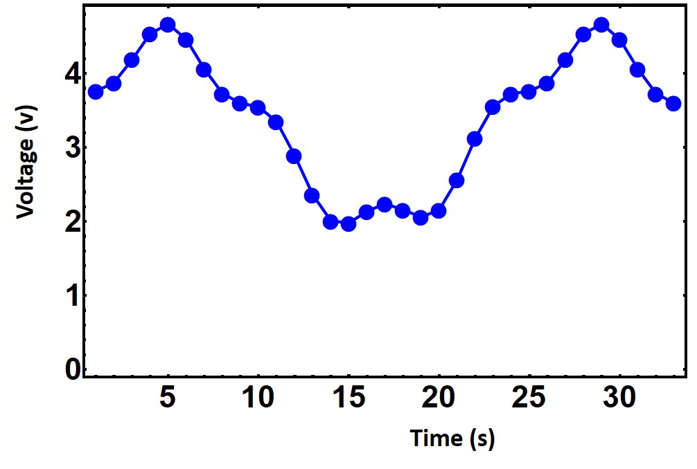
You can see the raw data in the mathematica notebook and the data is collected every 1ms. So how should we start solving this problem? What else can we identify immediately that is different from before? This signal is periodic!!! Specifically it repeats over a period, \( T = 24 \, \text{ms} \). So that will be our period and we will only select those points in that period for our DFT.

So we know as well that:
- \( N = 24 \)
- \( \Delta t = 1 \, \text{ms} \)
- \( T = 24 \, \text{ms} \)

That's a really good start.

Additionally, we also know:
- Sampling frequency: \( f_s = 1000 \, \text{Hz} \)
- Nyquist Frequency: \( f_{\text{Nyq}} = 500 \, \text{Hz} \)
- Fundamental frequency of the DFT: \( \Delta f = 42 \, \text{Hz} \)

Now let's calculate the DFT for this signal. To do that we need the Harmonic Coefficients, and instead of integrals we need to use summations:

$$
A_n = \frac{2}{N} \sum_{r=1}^{N} y(r \Delta t) \cos\left( \frac{2\pi r n}{N} \right) \quad n = 0, 1, \ldots, \frac{N}{2}
\]

$$
B_n = \frac{2}{N} \sum_{r=1}^{N} y(r \Delta t) \sin\left( \frac{2\pi r n}{N} \right) \quad n = 1, 2, \ldots, \frac{N}{2} - 1
\]

The same math follows as the previous example. Look at the mathematica notebook to check your answers.

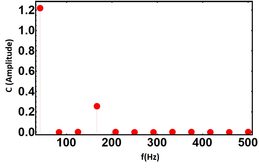
Note again I have converted the x axis into cyclic frequency. How do I get these values? What is my \( \Delta f \) spacing?

Well that is simply the lowest frequency or the fundamental frequency which we have already calculated above. You should note here that the frequency resolution here is again quite poor — you should be worried about spectral leakage.

DFT Fourier Series Reconstruction

We've done the hard part, we solved for the Harmonic coefficients so now to plot the Fourier Series for this DFT what equation should we use? This one below of course,

$$
y(t) = \frac{A_{0}}{2} + \sum_{n=1}^{\frac{N}{2}} \left[ A_{n} \cos(2 \pi n \Delta f t) + B_{n} \sin(2 \pi n \Delta f t) \right]
\]

So we have all the values we need to solve, plug into this equation and plot as seen below:

The blue points are our experimental data and the red line is our DFT calculated Fourier Series above. The fit looks nice so it looks like we sampled the curve sufficiently to reproduce the data.

Checklist: How to Accurately Sample a Discrete Signal

To accurately sample a discrete signal, do the following and you will be fine:

- Estimate the highest frequency in the signal and make sure that \( f_s \) is more than twice as large as that frequency.
- If you are forced to pick a Nyquist frequency less than the highest frequency in the signal, use a low-pass filter to block frequencies greater than the Nyquist frequency so those higher frequencies will not be aliased into your results.
- Estimate the lowest frequency in the signal or estimate the frequency resolution needed to accurately resolve the frequency components in the signal. Then choose the number of points in the sample \( N \) to yield the desired \( \Delta f = \frac{f_s}{N} \) at the previously determined value of the sampling frequency \( f_s \).