Chapter 1: Atomistic Structure of Materials

Topics Covered in this Class

Part I: Structure, Linear Elasticity, Stress and Strain Using Tensor Notation, Stress and Strain Transformations
Part II: Anisotropic Materials, Linear Viscoelasticity, Beams, Buckling, Plasticity
Part III: Strengthening Mechanisms, Creep, Deformation Mechanism Maps, and Fatigue and Fracture

The Materials Tetrahedron

The four corners of the Materials Science and Engineering Tetrahedron are: Structure, Processing, Properties, Performance. At the center is a combination of Characterization/Modeling/Experimentation.

A couple of quick examples: if you process sheet metal by cold rolling you change the structure and induce more dislocations in the material. This in turn will change the yield strength (property) and thus the performance of that sheet metal in the application of interest. As materials scientists, at the core of what we do is try to characterize material with experimentation and simulation to better understand this materials tetrahedron and to eventually reach a point where we can begin to predict some material responses.

Different Types or Classifications of Materials

- Metals
- Polymers
- Ceramics
- Composites
- Active Matter
- Piezoelectric
- Shape Memory Alloys
- Ferromagnetic Materials

Material Properties

- Thermal
- Magnetic
- Optical
- Electrical
- Structure

In this course we are going to focus in particular on Mechanical Properties!! However, as you are about to see in Materials Science, many properties are interrelated. One of the fundamental concepts we will see illustrated over and over again in this class is that structure will dictate properties.

Intra and Inter Molecular Bonding

Intramolecular Forces/Interactions

When it comes to binding and types of intramolecular interactions it is all about the electrons. Elements that have no valence electrons or that have a completely filled outer shell are called the inert or noble gases. All other elements which do not have a completely filled outer shell have valence electrons and these electrons are the ones of import when it comes to bonding. Bonding is critically important as most of the structural, physical, and chemical properties are influenced or determined by the interatomic bonding.

For intramolecular interactions we will typically deal with:

- Covalent (5 eV or about 200 kT)
- Ionic (1–3 eV or ~80 kT)
- Metallic (0.5 eV or ~20 kT)

Let’s talk a little bit about why bonding occurs. Well, it all goes back to Gibbs: the energy of the set of bonded atoms is lower than the isolated atoms.

Introduction to Thermodynamics

Ideally you have all taken one or two thermodynamics courses (the more the better). However we will take the time to review the essential concepts from thermodynamics that will be relevant to our discussion of the mechanical behavior of materials. Moreover, we will focus primarily on always keeping a strong physical intuition on what is occurring in a problem/process and how to relate that conceptually to concepts of thermodynamics and free energy. Thus, aside from this lecture, we will not spend a copious amount of time defining or deriving key thermodynamic quantities but instead focus on some key concepts and equations and relating how that impacts the mechanical properties of materials.

The Key Ideas for Thermodynamics in This Course

The fundamental equation that we will be working with when we talk about thermodynamics is Gibbs free energy:

\[G = U + PV - TS = H - TS\]

or more often we are interested in changes in Gibbs free energy:

\[\Delta G = \Delta H - T \Delta S\]

where \(U\) is the internal energy, \(T\) is the temperature, \(S\) is the entropy, \(G\) is the Gibbs free energy, \(P\) is the pressure, \(V\) is the volume, and \(H\) is the enthalpy.

One of the fundamental concepts in thermodynamics that we will continuously discuss is the competition between enthalpy and entropy. The competition between enthalpic interactions/contributions vs. the penalty or change in entropy will come up over and over again.

The focus of thermodynamic studies involves finding the state of a system/process at equilibrium. This occurs when the free energy is minimized, which occurs when the derivative of the free energy (with respect to externally applied forces) is set to zero.

When are we as humans at 0? When we are dead — we are non-equilibrium active matter!!

Also remember that a spontaneous process will occur when the change in free energy is less than zero.

Entropy Refresher

Now when thinking of entropy, typically the term that is often used to describe what entropy is physically is “disorder.” But this is a somewhat rudimentary way of conceptualizing entropy. As opposed to disorder, I would suggest to instead think of entropy (at least configurational or conformational, not vibrational yet) as the number of possible microstates that a system can exist in.

The entropy can be calculated using the following expression by Boltzmann (engraved on his tombstone):

\[S = k \ln \Omega\]

where \(\Omega\) is the number of microstates or configurations.

First Law of Thermodynamics

To do this we need to go back to the First Law of Thermodynamics. The First Law of Thermodynamics states that the increment of change in the internal energy of a system is equal to the heat (either into or out of the system) plus the increment of work (performed on or by the system). The first law of thermodynamics is thus a law of energy conservation. Energy is never destroyed!

$$
\begin{aligned}
dU &= \delta q + \delta w \\
dU &= dq + dw
\end{aligned}
\]

where q is heat, and w is the work term. Note here that dQ is the exact differential but the δ is an inexact or imperfect differential, i.e. it is path dependent. As a result I will typically just use the exact differential form for this class. There is also some confusion on the sign of heat and work. In this class we will say that heat transferred into a system will have a positive value and work done on a system will also have a positive value.

Second Law of Thermodynamics

The second law of thermodynamics states that the total entropy of an isolated system can never decrease over time. The second law confirms the existence of state functions or path independent functions and is concerned with the direction of natural processes. There are a couple of statements about the second law of thermodynamics. Clausius states that heat never spontaneously flows from an object at a lower temperature to one at higher temperature. Kelvin states that it is impossible to continuously perform work by cooling a system below the temperature of its surroundings. And perhaps the key statement is that the entropy of the universe (system and surroundings) must increase in any spontaneous process. It will only remain constant in a reversible process. IT IS NEVER NEGATIVE!!!

Let's think about an example for hydrostatic pressure work where we push a plunger extremely slowly so that we are at equilibrium at all times. For this the process is reversible and we can evaluate the exact differential. And for reversible processes we can relate entropy to heat transfer via the following equation

\[dQ = T dS\]

where S is entropy. Now before we get back to writing the full differential forms of free energy let's talk about some different forms of work that we may encounter in this class.

Types of Work

Work of Hydrostatic Pressure:

\[dw = -P \, dV\]

where P is the hydrostatic pressure and V is the volume, this is relevant for processes like pushing on a plunger or more importantly volume expansion.

Chemical Work:

\[dw = \mu \, dn\]

where μ is the chemical potential and n is the number of moles, this is relevant for many diffusion processes.

Work of Surface Energy:

\[dw = \gamma \, dA\]

where γ is surface tension and A is the area, this is critically important for coarsening and Oswald ripening.

Mechanical Work:

\[dw = \phi \, dq\]

where φ is electrical potential and q is the electric charge, very important for battery applications.

Elastic Deformation Work:

\[dw = \sigma \, d\epsilon\]

where σ is stress and ε is strain, very important for mechanical problems and rubber elasticity.

Typically there will be many other work terms which modify the internal energy of the system. Work terms can be generalized as so:

\[dw = \alpha \, d\beta\]

where α can be thought of as a generalized force and dβ is a generalized displacement. Additionally, each work term will consist of an intensive and extensive variable. An intensive variable will not scale or change with the size of system unlike an extensive variable which will change with the size of a system. For example pressure, temperature, chemical potential, stress, and electrical potential would all be intensive variables and volume, entropy, strain, number of particles, and charge would all be extensive variables. Typically the generalized force will be the intensive variable and the generalized displacement will be the extensive variable.

Interatomic Potentials

There are forces of attraction and repulsion between electrons and protons. The force F is related to the potential energy U by

\[F = - \nabla U\]

where ∇ is the gradient operator and will take the partial derivative of the function with respect to the dimensionality of the problem. There are many different equations or potentials that describe the interactions between atoms such as Morse, Born-Mayer, Van der Waals, etc. One of the most common is the Lennard-Jones (LJ) Potential which approximates the interaction between a pair of neutral atoms. It is popular due to the computational simplicity.

$$
U_{LJ} = 4\epsilon \left[\left(\frac{\sigma}{r}\right)^{12} - \left(\frac{\sigma}{r}\right)^{6}\right]
= \epsilon \left[\left(\frac{r_{o}}{r}\right)^{12} - 2\left(\frac{r_{m}}{r}\right)^{6}\right]
\]

where ε is the depth of the potential well, σ is the distance at which the inter-particle potential is zero, r is the distance between particles, and rₘ is the distance where the potential is minimized.

For ionic bonding Coulomb's law of electrostatic attraction can be helpful to describe the bonding and the force of coulombic attraction is given by

\[F_C = \frac{C e^2}{r^2}\]

where e is the charge of an electron, \(1.602 \times 10^{-19} \, C\), and C is Coulomb's constant \(8.988 \times 10^9 \, N m^2 C^{-2}\). The potential would then be

\[U_C = \frac{-A C e^2}{r} + \frac{B}{r^n}\]

Now that this digression is over we can get back to talking about the different types of intramolecular interactions and how to distinguish between covalent, ionic, and metallic interactions. The key to determining which type of bonding occurs is the valence electrons, specifically if they are gained, lost, or shared.

With covalent bonds there are valence electrons that are shared between adjacent atoms, which results in a pairing of electrons into localized orbitals and concentrating the negative charge between the positive nuclei. For ionic interactions we are typically dealing with atoms that have a different affinity for electrons, different electronegativities. A net transfer of charge can occur forming positively and negatively charged ions. These ions can form networks of ionic bonds held together by long-range coulombic interactions.

When the electronegativity is similar or the same between atoms the valence electrons are shared equally and the bond is purely covalent. When the electronegativity is very different the more electronegative atom withdraws nearly all the valence electrons and the bond is purely ionic. Thus electronegativity is how we distinguish between covalent and ionic interactions. In the intermediate case of electronegativity differences, bonds can have both covalent and ionic characteristics. We call these bonds polar covalent and one atom will have a partial positive and negative charge, as in HCl.

While there is no universally agreed upon cutoff value, in this class we will define an electronegativity difference of 0–0.4 to be non-polar covalent, 0.5–1.7 to be polar covalent, and greater than 1.7 to be ionic. In the case of metallic bonds, all atoms share their valence electrons and the nuclei form a positively charged array in a sea of delocalized electrons.

For soft matter the most common intramolecular interaction that we will deal with will be covalent interactions.

Intermolecular Forces/Interactions

As previously mentioned, intermolecular interactions are critical for many soft matter systems and there are several weak intermolecular interactions of interest, which include:

- Hard sphere potentials: the ability of atoms to effectively occupy space and repel at short length scales, quantum mechanical in nature
- Coulombic interactions: electrostatic attraction/repulsion between charged ions
- Lennard-Jones (LJ) potentials: induced dipole interactions between neutral atoms
- Hydrogen bonding: net dipole interactions
- The hydrophobic effect: a largely entropic interaction related to the structuring of water around hydrophobic interfaces
- Van der Waals force: includes London dispersion force, Debye force, and Keesom force which describe attraction and repulsion due to fluctuating polarization between nearby atoms/elements/particles, quantum mechanical in nature. Van der Waals forces decay as d⁻⁶

If you are interested in the origin of these interactions there is an excellent book by Israelachvili that I can recommend. The key thing to focus on is that all of these interactions have energies on the order of 1 kT, so thermal fluctuations can potentially break these bonds.

Structure of Crystalline Materials

A crystal structure is a periodic array of atoms that repeats over large distances. There is long-range periodic order, both long range translational and orientational order, in addition to short range order. Before we analyze crystal structures we first have to start off with a primitive lattice, lattice constants, interaxial angles, symmetries, point groups, and Bravais lattices.

Lattice, Primitive Unit Cell, Basis Vectors, Lattice Constants

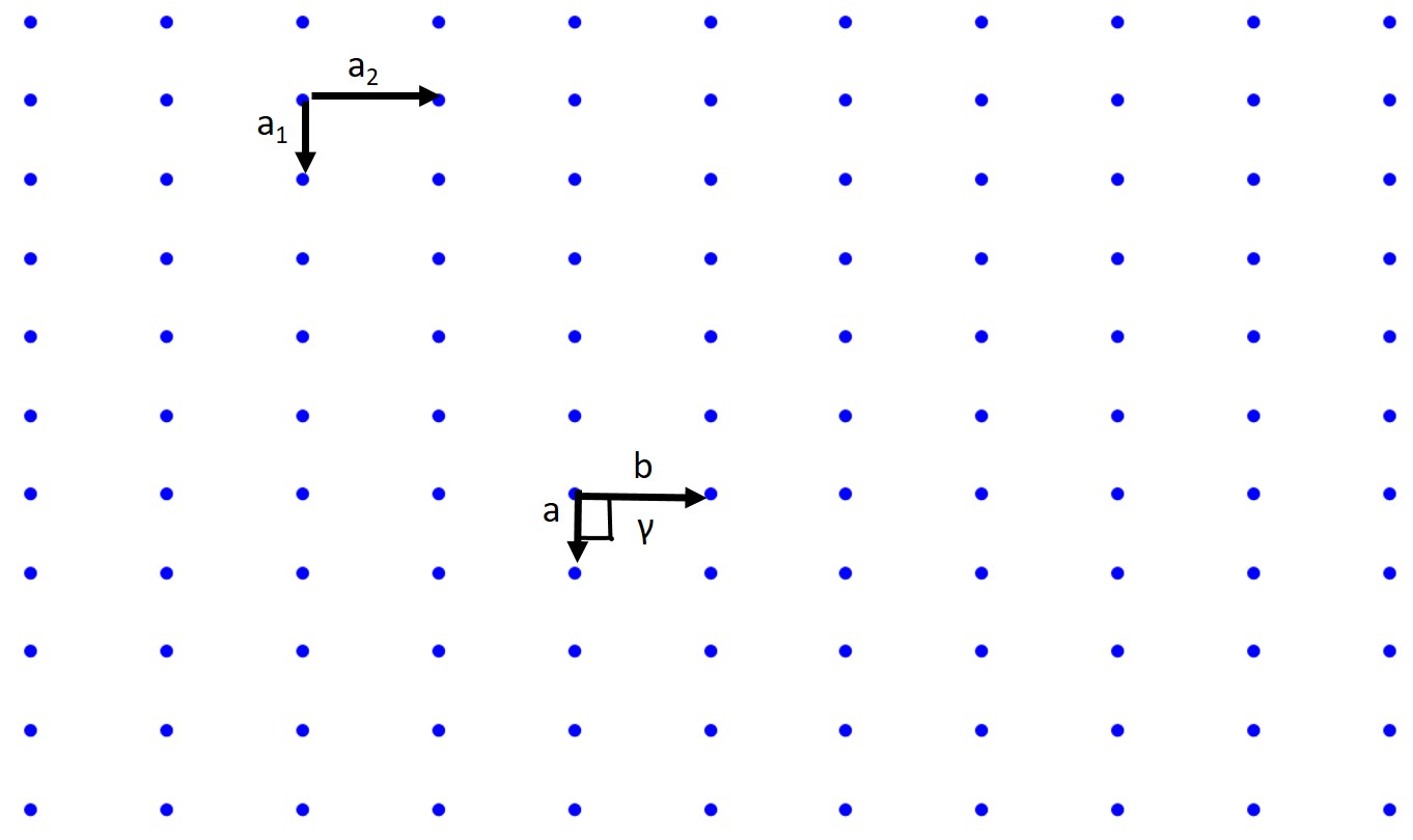
A lattice is a periodic array of points (atoms) in 1D, 2D, or 3D. Those points are lattice points. Let's start with the 2D case. A 2D lattice can be described by a primitive or unit cell which in turn is described by two lattice constants (a, b), two basis vectors (a₁ and a₂), and an interaxial angle γ. Once we have defined this we can pick any point in our 2D lattice as an origin and we can describe any point in our lattice with the previous values.

When we pick our basis vectors we pick the shortest lattice translation as a₁ and the second to shortest translation as a₂. The lattice constants are given by a = |a₁| and b = |a₂|. The interaxial angle γ is then defined. This also defines our primitive cell which will only contain a single lattice point.

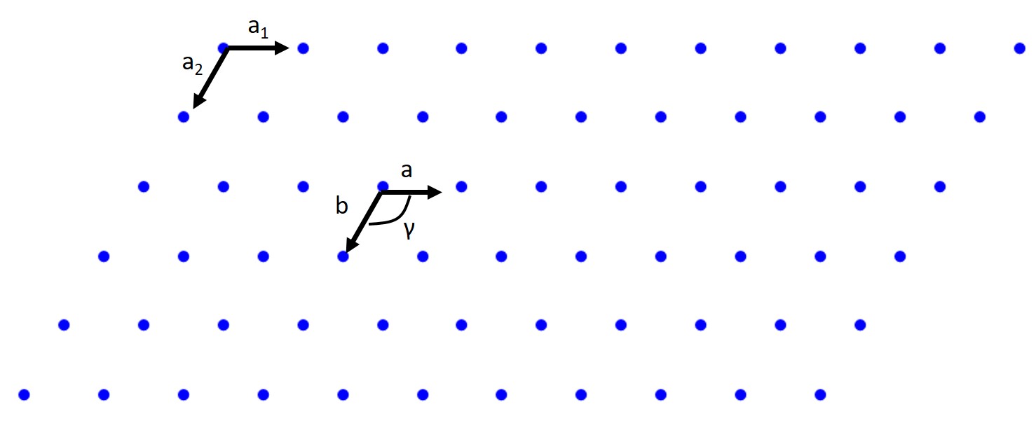
How about a rectangular lattice?

Associated with crystallography is a myriad of symmetry operations and we have just dealt with translational symmetry. There are also reflection or mirror symmetry, glide symmetry, rotational symmetry, and more. These topics are all important but we are not a crystallography class so we will not be covering them in detail, but you should know these concepts exist. There are also 230 space groups, 32 crystallographic point groups, 14 Bravais lattices, and 6 crystal systems.

Crystal Systems: Simple Cubic, BCC, FCC, HCP

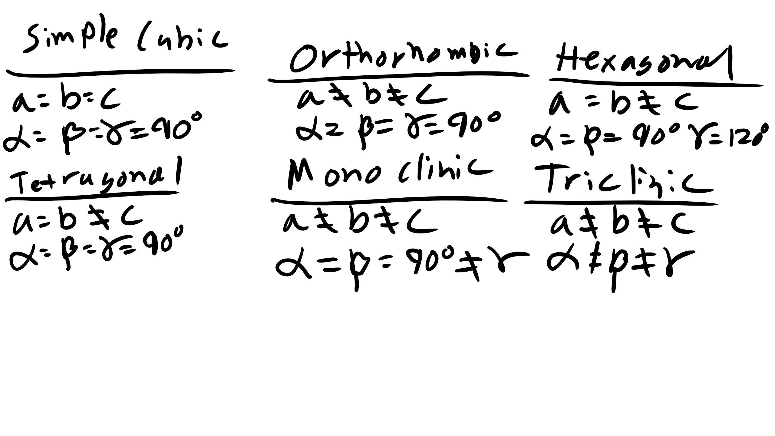
We are going to focus on the 6 crystal systems: triclinic, monoclinic, orthorhombic, tetragonal, hexagonal, and cubic. We will describe the unit cell, the primitive lattice vectors, and the interaxial angles.

You can see the rules and relationships between the lattice constants and the interaxial angles on the lecture slides.

Crystallographic Directions

When discussing crystals we will also have to specify crystallographic directions and planes. In order to refer to specific crystallographic planes or directions we need a labeling system to index them. This system is called Miller indices. A crystallographic direction is a vector denoted by [u v w]. u, v, and w are integers which correspond to the reduced projections along the x, y, and z axes, respectively. We always use [] for directions.

Example: draw the [100] direction. To draw the direction of a vector, pick an origin for the vector tail (the side without the arrow), then pick the ending point for the vector (the arrow). Subtract the arrow point from the tail point and the resultant vector must coincide with the direction you are trying to draw. Typically pick the origin as your origin.

How about the [111] direction?
What about [100]?
What about [1 -1 0]?
What about [222]?

Now a little more complicated: what is the vector below?

Crystallographically Equivalent Directions <hkl>

For a number of crystal structures there are several nonparallel directions with different indices that are crystallographically equivalent. This means that the spacing and number of atoms along each direction is the same. In cubic crystals [100], [-100], [010], [0 -10], [001], and [00 -1] are all crystallographically equivalent so we group them in a family denoted by angled brackets <100>.

Crystallographic Planes

For crystallographic planes we use Miller indices (h k l) which correspond to the x, y, and z axes respectively. Notice again that () are for planes and [] are for directions. <> is for families of directions. Families of planes are denoted with {}.

To draw planes, determine the intercepts. The intercepts are the inverse of the Miller indices. For example, the (111) plane:

For the (110) plane, if the inverse gives infinity, that means the plane is parallel to that axis. So the plane looks like this:

Another tricky problem is when the plane passes through the origin:

When a plane intersects the origin you must choose a different origin and repeat the procedure to determine intercepts and then Miller indices. Families of planes are denoted with {hkl}.

Here is a nice demonstration to visualize the Crystallographic Planes:
https://demonstrations.wolfram.com/C...CubicLattices/

Isotropic and Anisotropic

Up to now we have often assumed that material properties are the same in every direction. If materials behave in such a manner they are said to be isotropic materials. For many problems and theories in this course we will assume isotropy. This can often be the case for cubic structures. However, many materials are anisotropic, meaning that some material properties (mechanical, optical, kinetic, etc.) are different depending on the crystallographic direction you are investigating. For example titanium exhibits a larger modulus along the z-axis in the HCP structure than in the basal plane. This presents a significant problem when trying to superplastically form very thin titanium foil. A similar issue arises with magnetic properties of HCP materials as well. Also, real materials are not perfect single crystals — they are polycrystalline, made of many grains.

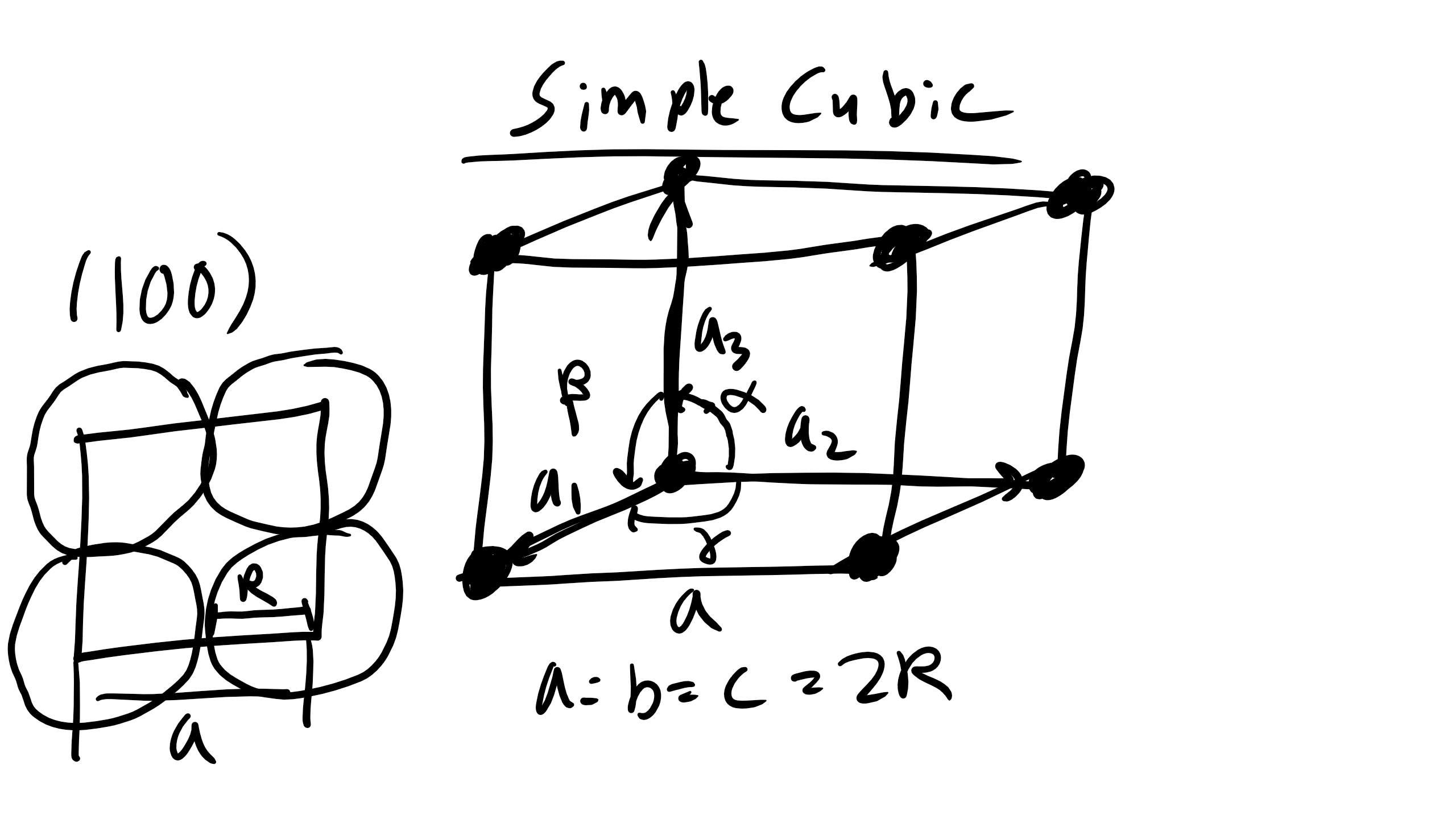
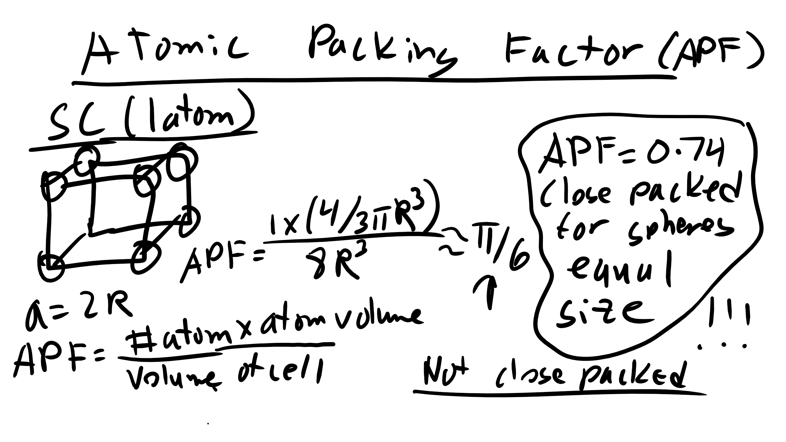
Simple Cubic (SC)

The simple cubic (SC), also called primitive cubic, is the structure for oxygen, fluorine, and others. It is described by the primitive lattice vectors a₁, a₂, and a₃ and interaxial angles α, β, γ. In SC all angles are 90° and a = b = c = 2R where R is the atomic radius.

How many atoms are contained in a simple cubic cell?
Answer: 1 atom (corner atoms shared by 8 unit cells).

How many nearest neighbors (NN)? 6.
How many second nearest neighbors (NNN)? 12.
What is the NN distance? 2R.
What is the NNN distance? \(2R\sqrt{2}\).

Atomic packing factor (APF): ratio of atom volume to unit cell volume. For SC:

\[\text{APF}_{SC} = \frac{\pi}{6}\]

Body-Centered Cubic (BCC)

The BCC structure is found in Li, Fe, V, Mo. It is described by lattice vectors a₁ = (a/2)[1 -1 1], a₂ = (a/2)[1 1 -1], a₃ = (a/2)[-1 1 1]. Angles are 90°. Geometry shows that

\[a = \frac{4R}{\sqrt{3}}\]

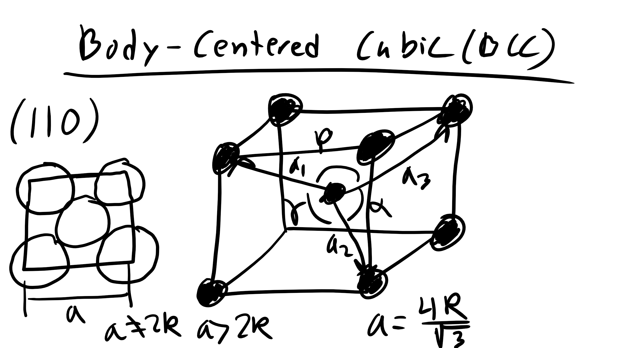
How many atoms per cell? 2 (1 inside + 8 corners shared).
How many NN? 8.
How many NNN? 6.
NN distance = 2R.
NNN distance = \( \frac{4R}{\sqrt{3}} \).
APF = 0.68.

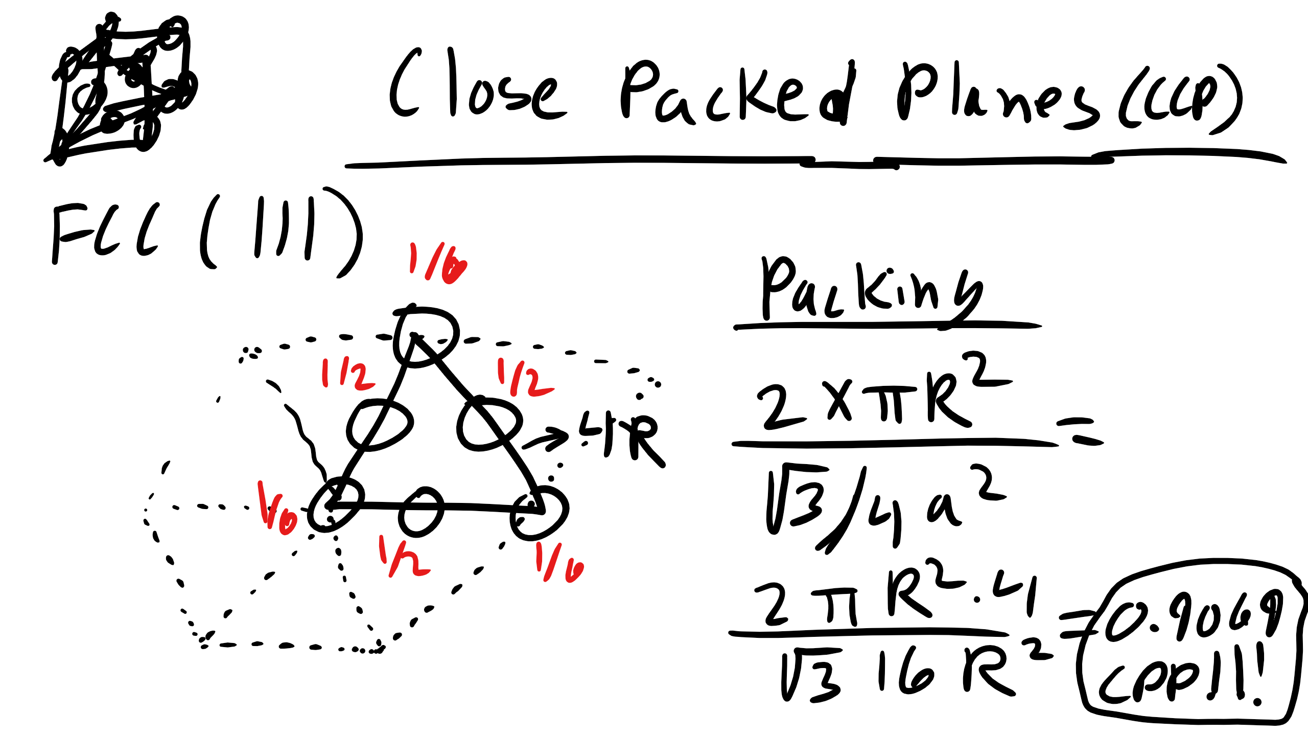
Face-Centered Cubic (FCC)

The FCC structure is found in Ni, Cu, Ca. Lattice vectors a₁ = (a/2)[0 1 1], a₂ = (a/2)[1 0 1], a₃ = (a/2)[1 1 0]. Angles 90°. In FCC:

\[a = 2\sqrt{2}\, R\]

Atoms per cell = 4 (8 corners shared + 6 faces shared).
Nearest neighbors = 12.
Second nearest neighbors = 6.
NN distance = 2R.
Second NN distance = \(2\sqrt{2}\,R\).
APF = 0.74 (the maximum possible packing for spheres of equal diameter).

Close-Packed Structures and Atomic Packing Factor

HCP and FCC both achieve the maximum APF of 0.74 and are called close-packed structures. FCC stacks ABCABC... indefinitely while HCP stacks ABAB... indefinitely.

Close-Packed Planes and Planar Density

A close-packed plane has a packing density ≈ 0.9069. Example: planar density of SC (100), BCC (110), FCC (111). Only close-packed structures can achieve close-packed planes, but often we care about the most closely packed plane even if not exactly 0.9069.

Close-Packed Directions

SC: <100>
BCC: <111>
FCC: <110>

Polymorphism/Allotropy

When materials have more than one crystal structure they are polymorphic. In elemental solids this is called allotropy. Examples: carbon (diamond, graphite, fullerenes, graphene), iron (BCC and FCC), titanium (HCP and BCC). Polymorphism is common and important in materials science.

Structure of Non-Crystalline Materials: Semi Crystalline and Amorphous

Examples include polymers, liquids, glasses, gases, liquid crystals, and many more. Up to this point we have focused only on crystalline materials because they are the simplest to characterize in terms of structure. However, many materials do not adopt a crystalline structure with short-range, long-range translational, and long-range orientational order.

With crystalline materials we were able to translate a unit cell to essentially infinity because we had short range order, long range translational order, and long range orientational order. In polymers, glasses, and liquid crystals typically we only have short range order (SRO) and perhaps some degree of long range order either translational or orientational but not both.

To describe these non-crystalline materials we use the dimensionless pair distribution function (PDF) or radial distribution function (RDF). This is also called the pair correlation function. It is our key descriptor for quantifying the SRO present in a material.

The PDF or RDF is defined as:

\[g(r) = \frac{1}{\langle \rho \rangle}\,\frac{dn(r, r+dr)}{dv(r, r+dr)}\]

where ρ is the average particle number density, dn is the number of particles counted in a small spherical shell sampling volume element of size dv at each distance r from a particle chosen as the origin. The number of particles in each shell is counted at each subsequent dr shell.

To get a smooth curve you want to pick dr much smaller than the particle radius and average over multiple origins. For perfect crystals the PDF shows sharp discrete peaks at interatomic spacings corresponding to the structure. For liquids you see a large first peak and then smaller peaks. The first peak corresponds to nearest neighbors, which can be calculated:

\[\langle NN \rangle = \langle \rho \rangle \int_{\text{peak}} g(r) \, 4 \pi r^2 \, dr\]

PDF can also be used to quantify SRO for glasses. Example: silica glass (also applies to thermoset polymers).