Chapter 3: Stress and Strain Curves

Lecture 3: Stress Stain Curves

Are you ready! We have talked enough about the atomistic length scale so now let's break some materials and look at stress strain curves right! Hold your horses for a second and lets cover some of the basics before we get started. Also as you can see from the title we will be going even further into the atomistic basis of elasticity, you will be glad we reviewed some material structure and bonding.

We are getting into the heart of this course which is the mechanical behavior of material which specifically refers to the material response to an applied load. This material response will depend on several factors including

- Internal forces and moments generated by external forces and moments
- Material properties: stiffness, strength, ductility, toughness, etc
- Component geometry

Specifically the mechanical behavior of materials and the mechanical properties of material will depend on the atomistic length scale we previously discussed. For example we will see today that stiffness will depend on binding energy, yield strength will depend on the presence of defects, etc.

But before we get into all this great material behavior lets do a quick review of internal and external forces. In previous classes we have discussed quite a bit about external forces but will also get into internal force more in-depth in this course.

We will also discuss quite a bit about moments which is the tendency of a force to cause rotation about a point or line and a moment can be defined as the cross product of a vector, \(\overline{r}\), from a point or line to the point where a force \(\overline{F}\) and note that this notation denotes a 1st rank tensor or a vector quantity as seen below

\[\overline{M_A} = \overline{r} \times \overline{F}\]

Also in 2D we can find the magnitude of the moment by multiplying the magnitude of the force by the perpendicular distance between a point A and the line of action of force

\[|M_A| = |F \cdot d| = r F \sin \theta\]

In this class we will always define CCW as positive and CW as negative. Also if a material extends we will consider that force and displacement positive and if it compresses then that is negative.

Additionally when we assume that we are in static equilibrium, we will set the sum of all the forces and all the moments to zero and that will eliminate both translation and rotation as seen below

$$
\begin{aligned}
\Sigma F &= 0 = ma \\
\Sigma M &= 0 = m \alpha r
\end{aligned}
\]

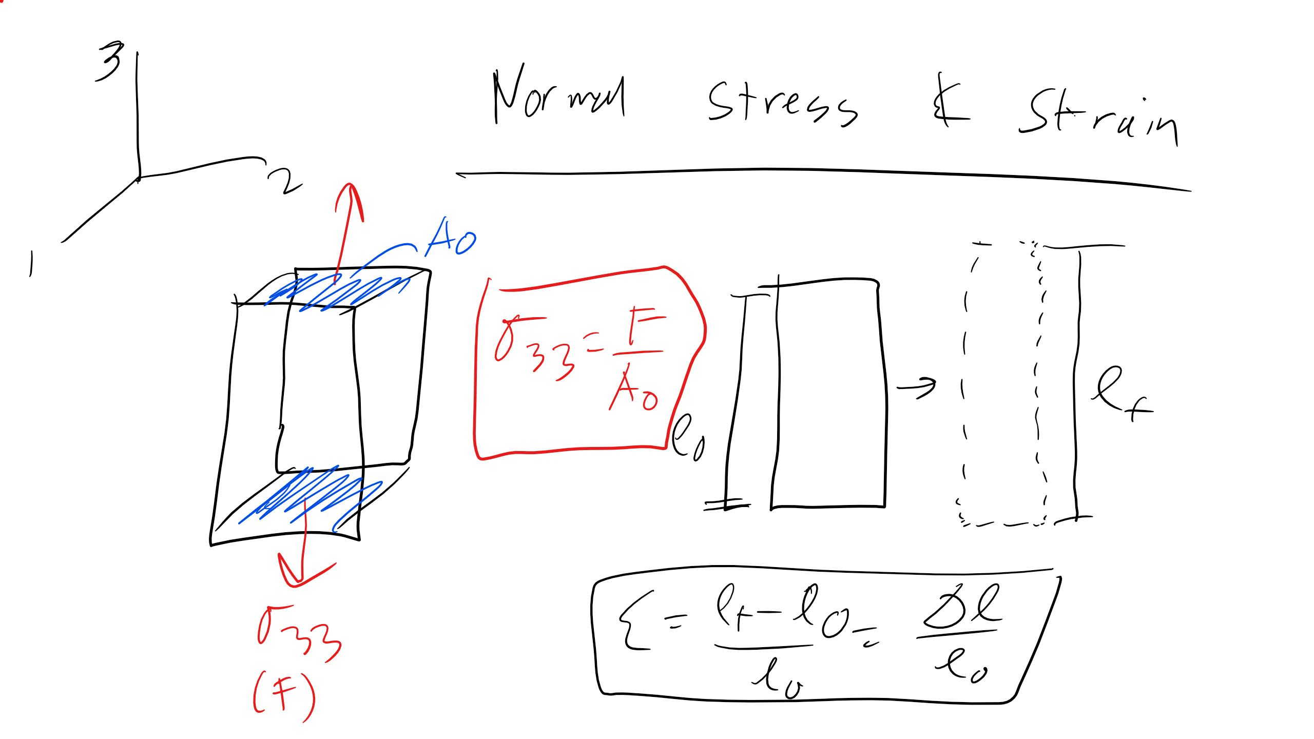
Normal Stresses

We will define normal stresses as those applied perpendicular to the area. We will define any forces, stresses, or strain in tension as positive and any forces, stresses, or strain under compression will be considered negative. It should be noted that to have uniform normal stress in a bar the load must act through the centroid of the bars' cross section as seen below

\[(\overline{x},\overline{y}) = \left( \frac{\int x \, dA}{\int dA}, \frac{\int y \, dA}{\int dA} \right )\]

At the end of a bar near the application of the load the stress will not be uniform unless the load is applied evenly over the area but becomes uniform at some distance, as stipulated by St. Venants Principle.

Normal Stress, \(\sigma\), is a force normalized by the area over which it acts and critically the force is normal to the cross sectional area over which it acts

\[\sigma = \frac{F}{A}\]

where \(F\) is force (in Newtons) and \(A\) is the original cross-sectional area. This is the definition of the engineering stress. The true stress would be normalized by the instantaneous area, more on this a little bit later. We will use the engineering stress primarily in this class.

Now when a force is applied to a material that material will deform and displacement will occur and this displacement is described by strain. Specifically here normal strain, \(\epsilon\), is defined as

\[\epsilon = \frac{l_f-l_o}{l_o} = \frac{\Delta l}{l_o}\]

where \(l_f\) is the final length after deformation and \(l_o\) is the initial length.

Hooke's Law for Isotropic Elastic Continuous Media

As we are all mechanical, civil, bio, computer science or really any engineers I am sure that Hooke's law is near and dear to your heart

\[F_s = -k \Delta x\]

Now you are all the experts with this expression but let me introduce you to another equation that is near and dear to the hearts of every material scientist and solid mechanics experts but can be very dangerous for students, so now I hate this equation

\[\sigma = E \epsilon\]

where \(E\) is the Young's modulus (sometimes you may see Y). Now, as you will see next lecture this equation is only applicable in the simple uniaxial stress state that you see here. This equation DOES NOT HOLD FOR OTHER COMPLEX STRESS STATES.

However, this equation is very relevant because when one produces a stress-strain curve the stress state is typically uniaxial tension using an instrument like our Instron machine in the laboratory. If there is nothing else that you take away from this course (and I know that you all will take much much much much more from this course) it is to master how to analyze a stress-strain curve. Whatever, engineering discipline that you eventually enter whether in academia or in industry you will be asked to work with a stress-strain curve, typically to select a material or to asses the material's performance.

Stress-Strain Curve:

When a material is placed under a stress state we will typically plot a stress-strain curve and that curve typically will have 3 distinct regions: I) Elastic, II) Plastic, III) Fracture.

I) Elastic Regime:

In the elastic regime the stress strain response is linear and the stress/strain is reversible, there is no hysteresis. This means you can recover the deformation upon unloading, i.e. the material will pop-back into place and the final length will be the same as the initial length upon unloading.

That describes the macroscopic mechanical response of the and if you look at what happens atomistically the bonds are being pulled but not broken and while dislocations are present they is no dislocation motion. This explains why there is no permanent or plastic deformation. You are just pulling on the bonds not breaking any bonds. Most materials behave linear and elastically at small strains, \(\epsilon < 0.002\).

Many materials will behave mechanically as isotropic materials, and again isotropic means that the properties are all the same in all directions, one example is a poly-crystalline metal with randomly orientated grains.

Now there are many other materials that will behave anisotropically, meaning that the properties are different along different directions, some of the most common examples would be wood, titanium, composites, etc.

In this regime we see that stress is linear and proportional to strain. More importantly, in this stress regime we have constitutive equations that relate stress to strain and we will introduce these equations in lectures to come. This is the only regime of the stress-strain curve where this is the case. In other regions, there is no fundamental equation that allows us to do so and instead we must rely on empirical equations and in this class we will focus more on trends and scaling parameters.

Typical values of Young's modulus for some materials can be seen below

- Diamond 1000 GPa
- Alumina 390 GPa
- Tungsten 340 GPa
- Steel 200 GPa
- Copper 110 GPa
- Concrete 30 GPa
- Al 6061 and Glass 69GPA
- Polethylene 0.2-0.7 GPa
- Rubbers 0.01-0.1 GPa

This is not a memorization class but it is always nice to have a couple of these material properties ready to impress at an interview. However, in this class a good rule of thumb is that if you are dealing with a ceramic you can approximate a Young's Modulus of 300 GPa, a metal to be 100GPa, and a polymer/biomaterial can vary between 100s of kPa to 10GPa so approximate it as 1GPa.

II) Plastic Regime:

Here you are plastically deforming the material. Macroscopically, once the material is stressed or strain such that the material enters the plasticity regime the deformation is irreversible. This means that the material will recover the elastic strain but the plastic deformation is irreversible so that the final length will be different than the initial length (it will be longer). There will be hysteresis upon unloading once the material enters this regime of the stress strain curve.

Atomistically, the plastic regime is distinct in that here the dislocation that are present in the elastic regime begin to become motile due to the stretching and breaking of bonds and resultant rearrangement of atoms. Additionally, in this regime dislocations and other defects can be created due to the rearrangement of atoms locally.

This regime initiates once the stress reaches \(\sigma_{y}\) which is the yield stress and and the yield stress reaches \(\epsilon_{y}\) the yield strain. This is the point where the stress-strain curve is no longer linear. Often times you will find in industry and sometimes in academia the yield stress is found using the 0.02% offset yield stress method in which a line with the same slope as the Young's modulus is drawn and the yield stress is determined at the point where the lines intersect. I personally have issues with this method so we will do a visual check and tack on some uncertainty to our measurement or justify with statistical methods. We can also see several other interesting points in this particular stress strain curve which does not represent all materials like the \(\sigma_{UTS}\) is the ultimate tensile strength. The ultimate tensile strength is defined as the largest stress value on the stress strain curve. In this particular curve it also indicates the onset of necking.

Necking is a type of plastic deformation that is denoted by a decrease locally in the cross-sectional area and forms a think neck as it's namesake indicates. The neck is formed from instabilities and heterogeneities in the material and due to the inherent decrease in the cross-sectional area of the cross-section when under tensile stress/strain because of conservation of volume considerations (as well as local variations in strain hardening more on this in a second).

The stress-strain behavior again is not governed by constitutive relationships and instead many of the relationships and behavior in this regime that we will discuss in later lectures is empirical (evidence based) in nature. We will discuss much more of this regime in later lectures to come. Lots of cool behavior in this regime.

III) Fracture:

This last regime is the regime that everyone is most interested in and the most fun to explore when running a tensile testing experiment and that is the loud pop that follows Fracture.

In this regime, catastrophic fracture occurs in a material. This is denoted by \(\sigma_{f}\) which is the fracture stress and the \(\epsilon_{f}\) is the fracture strain. Here macroscopically, the material cracks and new surfaces are created. Now this is very energetically unfavorable as we learned in our previous thermodynamics refresher, creating interfaces is typically very unfavorable. However, atomostically, the bonds are under immense strain near fracture and they are displaced far from their equilibrium distance so the elastic strain energy present in the bonds is incredible large and positive (very bad energetically). Even though, creating surfaces is unfavorable we can decrease the total free energy of the system by relieving this elastic strain energy by bond breaking and surface creation. This is the energy battle that determines when a material fractures, much more on this later. I know I know can we get to the end of the class so we can know everything about Mechanics yet, slow down but I appreciate the enthusiasm.

Fracture while the most fun practically is similar in nature to the plastic regime in that we do not have many fundamental equation that relate stress or strain here and inhomogeneties in the sample will cause fracture to be somewhat stochastic (random) in nature. But nevertheless we will press on.

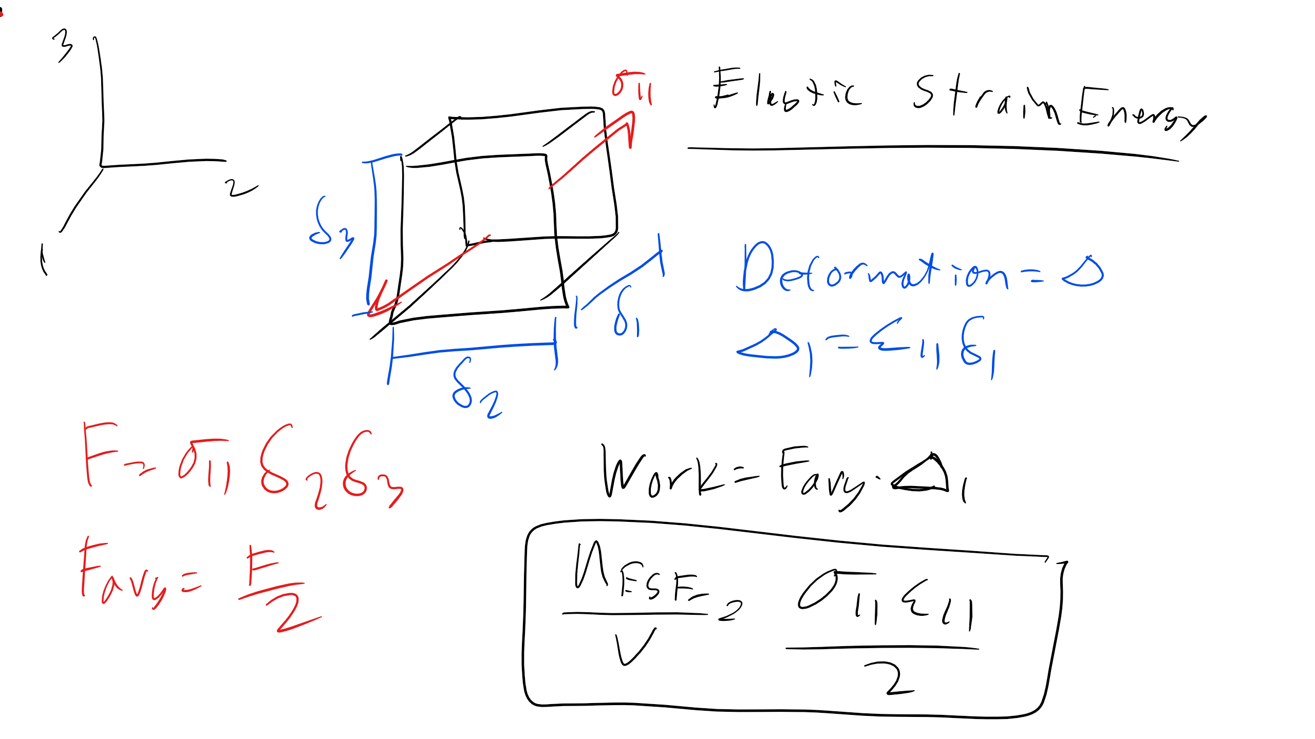
There are a couple of other material properties that we need to discuss at this point since we have reached the end of our stress-strain curve journey in terms of looking at the three regimes. We can also define the elastic strain energy you can define this value in terms of energy (Joule) or in terms of energy per unit volume. We can think about and calculate elastic strain energy in several ways, let's consider a representative volume element (RVE) a cube in this instance with a stress in the \(\sigma_{11}\) direction.

The force would simply be

\[F = \sigma_{11} \delta_2 \delta_3\]

Assuming that initially the force is 0 then the average force would simply be

\[F_{avg} = \frac{\sigma_{11} \delta_2 \delta_3}{2}\]

Thus if we consider that the deformation or

\[\Delta_{1} = \epsilon_{11} \delta_1\]

The the work would be assuming linear elasticity,

\[W = F_{avg} \Delta_{l} = \frac{\sigma_{11} \epsilon_{11} \delta_1 \delta_2 \delta_3}{2}\]

Or if we looked at the elastic strain energy per unit volume

\[\frac{dU_{ESE}}{dV} = \frac{\sigma_{11} \epsilon_{11}}{2}\]

Now this is one way to arrive at this expression, we can also simply look at the area under the curve which is

\[U_{ESE} = \int^{\epsilon_{y}}_{0}\sigma_{11} \, d\epsilon_{11} = \frac{\sigma_{11} \epsilon_{11}}{2}\]

[Figure: Elastic Strain Energy — file: ese.jpg]

Now that is a little bit easier and as you can see the expression matches with your previous expression. Also you can check for yourself that the units are indeed energy per volume, maybe a problem set question....no way too easy.

We can do something very similar to shear stress for example the stress applied on the top plane here would be

\[F_{avg} = \sigma_{12} \delta_2 \delta_3\]

The distance would then be

\[\Delta_{12} = \gamma_{12} \delta_3\]

Then then the work would be

\[W = F_{avg} \Delta = \frac{\sigma_{12} \gamma_{12} \delta_1 \delta_2 \delta_3}{2}\]

and thus

\[\frac{dU_{ESE}}{dV} = \frac{\sigma_{12} \gamma_{12}}{2}\]

In terms of strain energy we will also talk about how strain energy created a stress field in the crystal lattice around dislocations and we will explicitly calculate the strain energy associated.

One last value we should be aware of is toughness which is defined as

\[U_{T} = \int^{\epsilon_{f}}_{0}\sigma_{11} \, d\epsilon_{11}\]

This essentially the energy required to fracture a material, energy per volume to be precise. As you will soon see it is the total area under the curve both stress and the ability of a material to strain will determine toughness. Why is Kevlar a better body amour than steel? Let's discuss that right now but at this point we need to stop and make a clear point about the language that we have to use when discussing the material properties of materials. Word choice is critical here because they mean very different things. When we talk about the stiffness of materials we are talking about the Young's modulus of the material. The higher the Young's modulus the stiffer the material. When we talk about strength we are talking about the yield strength, the ultimate tensile strength, or the fracture stress or strength. We we are talking about how ductile a material is we are talking about the strain at failure. We also often talk about material resilience and toughness as well.

If a material is not as stiff it is called compliant, if a material is not strong it is weak, and if a material is not tough it is termed brittle.

Let's look at a few more stress-strain curves and talk about some differences that we can see just so that we can get a bit more acquainted. We will be going much much much more in-depth soon about some of these topics so don't worry, enjoy the overview while we can.

First let's break down some stress strain curves for different materials, specifically metals, ceramics, and polymers/biomaterials.

Now one thing you should have learned in materials science and what you will in fact learn here is that there are always counter-examples in materials science. But in general you will find that ceramics (glasses, tungsten, oxides, etc.) are typically very stiff but brittle. Many will exhibit little to no plastic deformation and many will fail suddenly at strains as small as \(\epsilon_f = 0.001\). Metals will be less stuff but can be more ductile and fail at much larger strains on the order of \(\epsilon_f = 0.1\). The ductility, stiffness, and strength depends on the bonding and the potential interaction as we will dive into more soon, so many soons. Polymers and biomaterials in general are much more compliant but are extremely ductile some polymers or more accurately elastomers can fail at strains as large as \(\epsilon_f = 5-10\) look at this that is approximately 4 orders of magnitude larger than for ceramics. This tells us a great deal about toughness as well, we can potential overcome a 3 order of magnitude differences in Young's modulus if we have such a discrepancy in the strain at failure.

True Stress-Strain curves

Now so far we have been dealing with engineering stress and strain curves and often this will be the more common stress-strain curve you will encounter. However, sometimes you may see a true stress-strain curve. This will not be too common but sometimes these curves are useful to describe material response at large deformations or they are utilized in plasticity studies because once the material plastically deforms the area is no longer constant.

Previously our engineering definition of stress and strain were as follows

$$
\begin{aligned}
\sigma_{eng} &= \frac{F}{A_o}\\
\epsilon_{eng} &= \frac{\Delta l}{l_o}
\end{aligned}
\]

However to describe true stress we can no longer use these definitions as beyond the elastic limit the specimen dimensions can be significantly different from their original values.

Thus we have to introduce new definitions of stress and strain, true stress and true strain. Here we find

\[\sigma_{true} = \frac{F}{A}\]

where \(A\) is the instantaneous area. We can relate the true stress to engineering stress by invoking a conservation of volume argument such that the following condition must hold true

\[A_o l_o = A l\]

Additionally we, we can re-write our engineering strain using this relationship such at

\[\epsilon_{eng} = \frac{l - l_o}{l_o} = \frac{A_o}{A} - 1\]

And thus we can also write

\[\frac{\sigma_{true}}{\sigma_{eng}} = \frac{F}{A} \frac{A_o}{F} = \epsilon_{eng} + 1\]

and finally we get the relationship for the plasticity regime that

\[\sigma_{true} = \sigma_{eng}(1 + \epsilon_{eng})\]

We can also write an expression to relate true strain to engineering strain in the plastic regime

\[d \epsilon_{true} = \frac{dl}{l}\]

Taking the integral

\[\epsilon_{true} = \int^{l_f}_{l_o} \frac{1}{l} \, dl = \ln \frac{l_f}{l_o}\]

Now to relate this expression to engineering strain we have to utilize the volume conservation expression we previously utilized and we can write the expression here

$$
\begin{aligned}
\frac{l}{l_o} &= e^{\epsilon_{true}} = \frac{A_o}{A} = 1 + \epsilon_{eng}\\
\epsilon_{true} &= \ln(1 + \epsilon_{eng})
\end{aligned}
\]

Another parameter that we will introduce here that you will often see in literature and particularly in polymers is the extension ratio \(\lambda = \frac{l}{l_o}\) and this will allow us to re-write true stress and strain quite simply

$$
\begin{aligned}
\sigma_{true} &= \sigma_{eng} \lambda \\
\epsilon_{true} &= \ln \lambda
\end{aligned}
\]

Now this expression holds true up to necking. After which the strain is non-uniform and computing the true stress-strain curve is no longer meaningful after necking. However, if we were able to instantaneously measure the necked area we could generate an entire stress-strain curve as our relationship for true strain would be

\[\epsilon_{true} = \ln \frac{L}{L_o} = \ln \frac{A}{A_o}\]

Often for ductile metals you will typically see a power-law relationship for the expression for true stress and true strain

\[\sigma_{true} = A \epsilon^n_{true} = \log \sigma_{true} = \log A + n \log \epsilon_{true}\]

The parameter \(n\) is referred to as the strain hardening parameter, more on this a bit later but many ductile metals vary from \(n=0.02-0.5\). But speaking of strain hardening and strain softening....

Strain Hardening, Strain Softening, or Elastic-Perfectly Plastic

Some materials can strain harden, strain soften, or behave elastic-perfectly plastic for example we can describe the true stress beyond the yield stress as

\[\sigma_{y} = \sigma^{o}_{y} (1 + \epsilon_{true})^n\]

The materials will behave as follows depending on the strain hardening exponent \(n\)

- Strain Hardening \(n>0\)
- Elastic-Perfectly Plastic \(n=0\)
- Strain Softening \(n<0\)

We can actually see how the true stress and strain curves compares the engineering stress and strain curve below

Now you are all experts in everything stress-strain curves so we can end the class.....not so fast all of this that we have discussed is for a very very specific stress-state uniaxial tension. Unfortunately this is not a common stress state so we need to go much deeper and dive into the tensorial definition of stress and strain.