
Chapter 6: Goodness of Fit Hypothesis Testing
- Page ID
- 99726
Here you can find a series of pre-recorded lecture videos that cover this content: https://youtube.com/playlist?list=PLSKNWIzCsmjA4X-lkFzKySeumT1S5t3om&si=vYb0kaHmSIrHBBGn
So far we have discussed Gaussian/normal distributions, t-distributions, and some other distributions briefly. Another useful and common distribution you may come across is the chi-square (\(\chi^2\)) distribution. This distribution is distinct from the ones that we have dealt with previously as you can see below first we can see it has the shape of a right-skewed curve.
The area under the curve is again 1.0 same as before and and as the ν becomes large the distribution approaches a symmetric distribution resembling the normal distribution. \(\chi^2\) is often referred to as a goodness of fit test statistic is:
\begin{equation}
\chi^{2} = \sum \limits_{i=1}^k \frac{(O_{i} - E_{i})^2}{E_{i}}
\end{equation}
where Oi is the observed data, Ei is the expected data, k is the total number of variables being compared, and ν = k − 1 − r, where r is the number of fitting parameters...more on this later. We will see in several examples that you can also think of this k as counting the number of possible outcomes. k IS NOT THE NUMBER OF SAMPLES. It is critical to remember that k is not n. The \(\chi^2\) is a right tailed test for hypothesis testing since \(\chi^2\) is a positive value. Also when the observed data approaches the expected data the value of \(\chi^2\) approaches zero.
Let’s do a quick example right here to get a sense of when and how we can utilize this distribution with an example.
Flipping coins
Let’s start off with flipping a coin. I asked one of my undergraduate research students to flip a coin 500 times as I was interested to see if my coin had any weight imbalance that would lead to a non-stochastic result in coin flipping, I know I am very mean. But my student flipped the coin 500 times and found 286 heads and 214 tails. Is this coin fair or true using a confidence level of 95%?
So to start with this problem I want to first point out this issue of fair or true. That just means that the probabilities or outcomes are what we expect. For example flipping a coin should be stochastic or random and thus the probability of getting heads or tails should be 50:50 if we see a significant deviation from our hypothesis test then we know that something has gone wrong. So let’s get started first what is k here?
It is not 500! The number of possible outcomes is the coin will be either head or tails so k = 2. For the rest we just follow our hypothesis testing procedure
\begin{eqnarray}
H_{0}: Frequencies & are & same\\
H_{a}: Frequencies & are & different \\
\chi_{exp}^{2} = 10.368\\
\chi_{0.05,1}^{2} = 3.841
\end{eqnarray}
We are in the reject region so these coins are not fair, see I was right.
Note again that for this distribution we will always be dealing with a right tailed test due to the shape and nature of the distribution.
Fun with Random Numbers
As an expert Mathematica coder you generate 300 random numbers in the range from 0-10 and you get the following seen in the Mathematica Notebook

Figure \(\PageIndex{1}\): Random Number Generator Distribution 0-10.
Does the distribution differ significantly from the expected distribution at the 1% significance level?
\begin{eqnarray}
H_{0}: Frequencies & are & same\\
H_{a}: Frequencies & are & different \\
\chi_{exp}^{2} = 17.753\\
\chi_{0.01,10}^{2} = 23.209
\end{eqnarray}
We do not reject that hypothesis. We can always trust in Mathematica! Note: Mention anecdote about Mathematica random number failing.
Why Am I So Old No Student Has Seen Casino
Ace Rothstein suspects a player at his casino of cheating so he asks you to test if his dice are true and he gives you the following data set for the outcome of rolling two 6 sided die. Ace wants to make sure there is no cheating so you can see he ran this experiment 800 times, he appreciates large data sets to work with as seen below
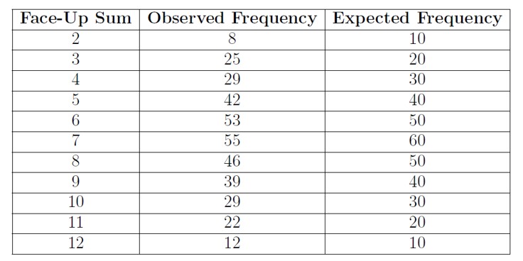
Figure \(\PageIndex{2}\): Dice Roll Distributions.
Determine if the dice are true at a 99% confidence level.
\begin{eqnarray}
H_{0}: Frequencies & are & same\\
H_{a}: Frequencies & are & different \\
\chi_{exp}^{2} = 297.826\\
\chi_{0.01,10}^{2} = 23.209
\end{eqnarray}
So as you can see we fall in the reject region....uh oh!
Are My Rolling Velocities Normally Distributed?
You cannot escape my rollers!! Let’s go back to our data set and see if our rolling velocities are normally distributed.
If you remember we found that sample mean rolling velocity was 2.938 \(\frac{\mu m}{s}\) with a standard deviation of 0.376 and we measured 138 samples. We find that there are 15 measurements with a velocity greater than 3.4 same units, 43 less than 2.8. We also find that there are 37 measurements between 2.2 and 2.8 and finally 136 measurements between 2 and 4.
Are the velocities normally distributed at the 5% significance level?
As usual we need to find what the expected values if they were normally distributed. To do this we need to go back to our old friend the Z-Table and calculate z values and look up areas. So let’s break this problem up.
1. Greater than 3.4
\begin{eqnarray}
z = \frac{3.4-\overline{x}}{S_x} = 1.23\\
A_{1} =0.5-0.3907=0.1093\\
E_{1} = n \cdot A_1 \approx 15
\end{eqnarray}
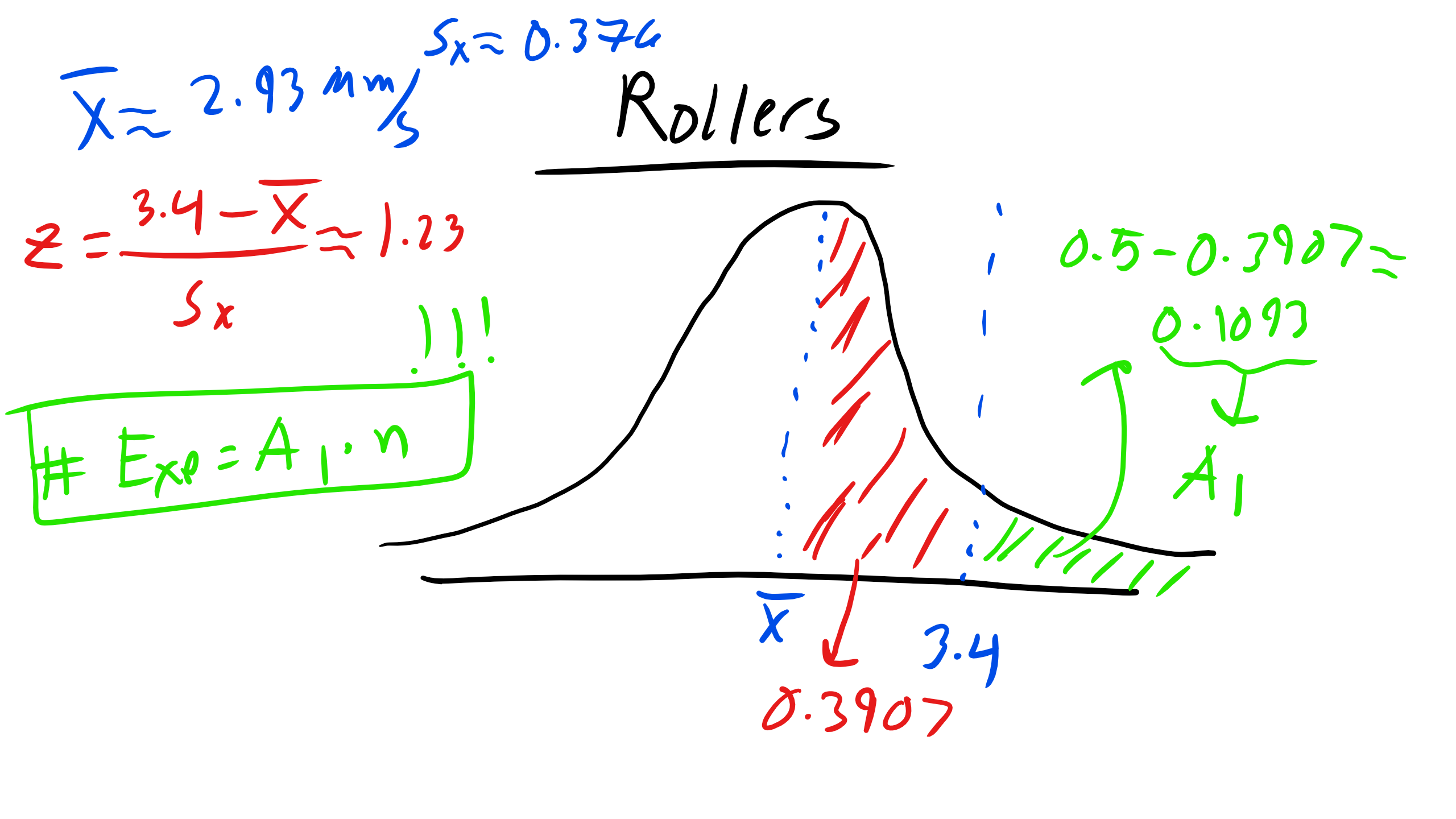
Figure \(\PageIndex{3}\): Solving for Area 1.
2. Less than 2.8
\begin{eqnarray}
z = \frac{2.8-\overline{x}}{S_x} = -0.37\\
A_{2} =0.5-0.1443 = 0.3557\\
E_{2} = n \cdot A_2 \approx 49.1
\end{eqnarray}
3. Between 2.2 and 2.8
\begin{eqnarray}
z = \frac{2.2-\overline{x}}{S_x} = -1.96\\
A_{3} =0.475-0.1443=0.3307\\
E_{3} = n \cdot A_3 \approx 45.6
\end{eqnarray}

Figure \(\PageIndex{4}\): Solving for Area 3.
4. Between 2 and 4
\begin{eqnarray}
z = \frac{2-\overline{x}}{S_x} = -2.49\\
z = \frac{4-\overline{x}}{S_x} = 2.82\\
A_{4} =0.4936+0.4976=0.99\\
E_{4} = n \cdot A_4 \approx 136.7
\end{eqnarray}

Figure \(\PageIndex{5}\): Solving for Area 4.
Whew....that was quite a bit of work but now we can actually go ahead and perform our analysis via hypothesis testing but first let us figure our the degrees of freedom, ν. We know the possible outcomes or variables k we are dealing with is 4 since we have 4 bins in our histogram. Now the question is what is r. Well when we are talking about a distribution or fitting r is the number of parameters used to fit the distribution, so when looking back at the Gaussian equation we fit based on values we calculate for µ and σ. If we were working with a 20th order polynomial fit r would be 20 but in this example for Gaussian distributions we have r = 2 thus we know that ν = 1.
\begin{eqnarray}
H_{0}: Frequencies & are & same\\
H_{a}: Frequencies & are & different \\
\chi_{exp}^{2} = 2.4\\
\chi_{0.05,1}^{2} = 3.841
\end{eqnarray}
So We do not reject.
Goodness of Fit
Most data is Gaussian however there are certain data sets that are not approximated well by the Gaussian distribution. The most well know example begin perhaps fatigue strength data which is approximated using the Weibull distribution. So some estimate of the goodness of fit should be made before any critical decisions are based on statistical error calculations.
There is no absolute or cure all check in producing a figure of merit, at best a qualifying confidence level must be applied with final judgment left to the experimentalist. The quickest and easiest method is to eyeball the results but this is problematic and very subjective. Another method would be to graphically check using a normal probability plot.
Yet another methods is to test for goodness of fit based on the \(\chi^2\) distribution although this requires considerable data manipulation and does not lend itself well to small samples of data.
Some limitations of this technique are that originally determined values must be numerical counts and integer frequencies, frequency values, should be equal to or greater than unity and there should be not unoccupied bins, and the use of \(\chi^2\) is questioned if 20% of the values in either the expected or original ins have counts less than 5.
Now you may have hear of another \(\chi^2\) test that gives you information about how variables can be correlated, don’t worry we will get to that later.