
1.8: Instrumentation and Laboratory
- Page ID
- 52873

At this point we need to shift gears and focus on a few practical aspects, the sort of things we might deal with in an electrical laboratory. It is one thing to discuss abstract concepts such as voltage and current, and quite another to deal with them in the real world.
Sources
For starters, let's consider the idea of power sources, that is, devices that can produce reliable, stable and constant voltages and/or currents. As mentioned previously, a battery approximates an ideal voltage source. The problem, of course, is that batteries only last a finite period of time and their voltage begins to sag after being used for a while. Also, their voltage is fixed and not adjustable. An adjustable voltage source would be much more flexible in a laboratory.
To address this problem, most electrical labs use a variable DC voltage supply in place of simple batteries. These sources typically are adjustable from 0 to 25 volts or higher and can produce one amp of current or more. An example is shown in Figure 2.8.1 . This particular unit has two main outputs plus a third auxiliary output. All outputs are independent, meaning that the voltage of each can be set independent of the others. Further, the two main outputs offer programmable current limiting. This feature can be thought of as a programmable fuse or circuit breaker: it limits the amount of current a circuit can draw to some preselected level. It is worth noting that even if a source is rated for, say, two amps, that only refers to the maximum value that can be drawn; that is not the current that it would produce by default.
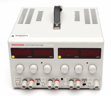
Figure 2.8.1 : A multi-output adjustable DC voltage supply.
Multiple output power supplies are usually wired in a “floating” form, meaning that the negative terminal is not tied back to earth ground. A separate connector is presented (usually green) that is tied back to earth ground if it is needed. Having floating supplies gives the user much more flexibility. For example, two floating supplies can be wired in sequence to create a single higher voltage. They can also be wired to present a positive voltage and a negative voltage. The unit shown in Figure 2.8.1 also features twin LED displays for voltage and current for each of the main outputs. It is worthwhile to point out that the color coding used for electronic equipment is not the same as that used for residential wiring in North America. The electronics standard is that the common or ground terminal is black while the “hot” or positive terminal is red.
While there are a large number of makes and models of affordable laboratory DC voltage sources available, the same is not true of DC current sources. This is not usually a problem. As we shall see in upcoming work, it is possible to emulate a constant current source using a voltage source and some attached components.
Schematic Symbols
Clearly, it would not be practical to create circuit drawings (schematics) using pictures of the actual devices. Instead, we use simple schematic symbols to represent them. There are two widely used schemes: ANSI (American National Standards Institue) and IEC (International Electrotechnical Commission). For many electronic components the ANSI and IEC versions are the same, but there are notable differences. ANSI tends to dominate in North America (surprise!) while IEC tends to dominate elsewhere.
Figure 2.8.2 shows the symbols for DC current and voltage sources. The long bar at the top of the voltage source is the positive terminal while the shorter bar at the bottom denotes the negative terminal. For the current source, the arrow points in the direction of conventional current flow. If the source is adjustable, it will often be shown with a diagonal arrow drawn through it. In some schematics, a DC voltage source will simply be drawn as a “connection dot” or node with the voltage labeled. It is assumed that the other end of the source is tied back to the system common or ground.


Figure 2.8.2 : Voltage (left) and current source schematic symbols.
Speaking of ground, there are three different symbols used for a circuit's common connection point. These are: earth ground, chassis ground and signal or digital ground. These are shown in Figure 2.8.3 . Earth ground is used when the circuit common is tied back to true earth (e.g., to the third pin on an AC receptacle). Chassis ground is a more generic term which would represent a common reference point that did not go back to true earth (e.g., a portable device). Finally, digital or signal ground is used to distinguish between common points where they might be separated for noise or interference concerns (e.g., a sensitive analog signal common separate from a digital logic common).


Figure 2.8.3 : Schematic symbols for ground. (L-R) earth, chassis, signal.
The symbols for resistors and other resistive devices vary considerably between ANSI and IEC versions. ANSI uses a zig-zag line while IEC uses a simple rectangle. These are illustrated in Figure 2.8.4 . This text will focus on using the ANSI standard symbols for resistors. One final note about component values: As decimal points are easy to lose on photocopies or small display screens, engineering notation multipliers are sometimes placed in the position of a decimal point. For example, a 4.7 k \(\Omega\) resistor may be listed as simply 4k7.


Figure 2.8.4 : Schematic symbols for resistive devices. (L-R) resistor (ANSI), resistor (IEC), photoresistor, thermistor.
Measurement – The Digital Multimeter
Perhaps the most handy measurement device in the electrical laboratory is the digital multimeter, or DMM for short. These handheld devices are used to measure voltage, current and resistance; and depending on model may have other measurement capabilities as well. A pair of typical units are shown in Figure 2.8.5 .
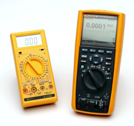
Figure 2.8.5 : Digital Multimeters.
Beyond the measurement functions of the DMM, perhaps the single most important characteristic is its accuracy. It is important to remember that no measurement device is perfect and there is always some uncertainly between what the device indicates and the true value of the parameter being measured. As a DMM uses a digital display, it has both finite range and resolution. As you might guess, the more digits the meter can display, the greater its potential accuracy. DMMs are commonly described as having 3 1/2 digits, 3 3/4 digits, 4 1/2 digits, and so on for their displays. A fractional digit is simply a leading digit that cannot go up to nine. By common use, the term “1/2 digit” means that the leading digit can be no more than one. A 3/4 digit specification typically means that the first digit can't be larger than three (it might also be four or even five as this terminology is not standardized)1 . To clarify, a 3 1/2 digit display is also referred to as a “2000 count” display. This is because there are 2000 possible values, from 0000 to 1999. Similarly, a 4 3/4 digit display is called a 40,000 count display because it has 40,000 possible values, from 00,000 to 39,000.
Using a 2000 count display as an example, the next question to ask is where to place the decimal point. This display could be set up to read from 0 to 1999 volts. For convenience, we would call that a “2000 volt scale”, meaning that the maximum voltage that can be displayed is approximately 2000 volts. With an otherwise perfect meter, the error can be as large as 1 volt because we have no way of indicating fractions of volts. To solve this limitation we could add other scales by shifting the decimal point. For instance, we could make a nominal “20 volt scale” which would range up to 19.99 volts, giving us resolution down to 10 millivolts. We could go further and make a 2 volt scale with a maximum of 1.999 volts and 1 millivolt resolution as well as a 200 millivolt scale with a maximum of 199.9 millivolts yielding a resolution of one-tenth millivolt. We might need to measure very large as well as very small voltages, so the scale setting is user adjustable.
It is important to use the lowest scale that can display the desired value otherwise a loss of resolution and accuracy will occur. For example, if we need to measure a voltage somewhere around five or six volts with this 2000 count meter, it should be set for the 20 volt scale. A lower setting, such as a 2 volt or 200 millivolt scale, will not be able to display the measurement and instead will indicate an overload condition (usually by flashing an abbreviated error message such as “Err” or “OL”). On the other hand, if the higher 2000 volt scale is used, the meter will only be able to resolve the measurement to the nearest volt. Indeed, this is so important that some meters have auto-ranging, meaning that they will automatically choose the scale setting to give the best result. The accuracy specification for a DMM is in two parts. The first part is the percent deviation around the measured value. The second part is the added number of counts.
The accuracy specification for a typical 3 1/2 digit meter might be \(\pm\) 2% of reading plus 3 counts. To determine the range of possible values for a reading, first determine the percentage of the reading and then add in the number of counts (i.e., one count represents the resolution of the meter on that particular scale). The resulting value represents the uncertainty of the reading. It can also be visualized as an “error envelope” surrounding the displayed value. Somewhere in that envelope is the true value measured. This is shown in the following examples.
A 3 1/2 digit (2000 count) DMM has an accuracy specification of \(\pm\) 2% of reading plus 3 counts. On its 20 volt scale it measures 5.01 volts. Determine the uncertainty in this measurement.
On its 20 volt scale this meter can display up to 19.99 volts. Therefore its resolution, or single count value, is 0.01 volts. Thus, 3 counts is 0.03 volts. To this we add 2% of the reading of 5.01 volts, or 0.1002 volts. The total is 0.1302 volts or 130.2 millivolts. This represents the error envelope on either side of the reading. That is, the true value is within the range of 5.01 volts \(\pm\) 130.2 millivolts, or somewhere between 4.8798 volts and 5.1402 volts. In other words, the ambiguity is about 130 millivolts out of about 5 volts.
A 4 3/4 digit (40,000 count) DMM has an accuracy specification of \(\pm\) 0.1% of reading plus 8 counts. On its 4 volt scale it measures 3.0035 volts. Determine the uncertainty in this measurement.
On its 4 volt scale this meter can display up to 3.9999 volts. Therefore its resolution is 0.0001 volts or 0.1 millivolts. 8 counts is 0.8 millivolts. To this we add 0.1% of the reading of 3.0035 volts, or 3.0035 millivolts. The total is 3.8035 millivolts. This represents the error envelope on either side of the reading and the true value is somewhere between 2.9996965 volts and 3.0073035 volts. The ambiguity here is just a few millivolts out of about 3 volts. Clearly, this meter's level of ambiguity is much reduced compared to the meter used in Example 2.8.1 .
References
1You might rightly ask how it is that having just one numeral out of nine counts as “half” and three out of nine counts as “three fourths”. Well, that's marketing for you.