
4.2: Source Conversions
- Page ID
- 52908

\( \newcommand{\vecs}[1]{\overset { \scriptstyle \rightharpoonup} {\mathbf{#1}} } \)
\( \newcommand{\vecd}[1]{\overset{-\!-\!\rightharpoonup}{\vphantom{a}\smash {#1}}} \)
\( \newcommand{\id}{\mathrm{id}}\) \( \newcommand{\Span}{\mathrm{span}}\)
( \newcommand{\kernel}{\mathrm{null}\,}\) \( \newcommand{\range}{\mathrm{range}\,}\)
\( \newcommand{\RealPart}{\mathrm{Re}}\) \( \newcommand{\ImaginaryPart}{\mathrm{Im}}\)
\( \newcommand{\Argument}{\mathrm{Arg}}\) \( \newcommand{\norm}[1]{\| #1 \|}\)
\( \newcommand{\inner}[2]{\langle #1, #2 \rangle}\)
\( \newcommand{\Span}{\mathrm{span}}\)
\( \newcommand{\id}{\mathrm{id}}\)
\( \newcommand{\Span}{\mathrm{span}}\)
\( \newcommand{\kernel}{\mathrm{null}\,}\)
\( \newcommand{\range}{\mathrm{range}\,}\)
\( \newcommand{\RealPart}{\mathrm{Re}}\)
\( \newcommand{\ImaginaryPart}{\mathrm{Im}}\)
\( \newcommand{\Argument}{\mathrm{Arg}}\)
\( \newcommand{\norm}[1]{\| #1 \|}\)
\( \newcommand{\inner}[2]{\langle #1, #2 \rangle}\)
\( \newcommand{\Span}{\mathrm{span}}\) \( \newcommand{\AA}{\unicode[.8,0]{x212B}}\)
\( \newcommand{\vectorA}[1]{\vec{#1}} % arrow\)
\( \newcommand{\vectorAt}[1]{\vec{\text{#1}}} % arrow\)
\( \newcommand{\vectorB}[1]{\overset { \scriptstyle \rightharpoonup} {\mathbf{#1}} } \)
\( \newcommand{\vectorC}[1]{\textbf{#1}} \)
\( \newcommand{\vectorD}[1]{\overrightarrow{#1}} \)
\( \newcommand{\vectorDt}[1]{\overrightarrow{\text{#1}}} \)
\( \newcommand{\vectE}[1]{\overset{-\!-\!\rightharpoonup}{\vphantom{a}\smash{\mathbf {#1}}}} \)
\( \newcommand{\vecs}[1]{\overset { \scriptstyle \rightharpoonup} {\mathbf{#1}} } \)
\( \newcommand{\vecd}[1]{\overset{-\!-\!\rightharpoonup}{\vphantom{a}\smash {#1}}} \)
\(\newcommand{\avec}{\mathbf a}\) \(\newcommand{\bvec}{\mathbf b}\) \(\newcommand{\cvec}{\mathbf c}\) \(\newcommand{\dvec}{\mathbf d}\) \(\newcommand{\dtil}{\widetilde{\mathbf d}}\) \(\newcommand{\evec}{\mathbf e}\) \(\newcommand{\fvec}{\mathbf f}\) \(\newcommand{\nvec}{\mathbf n}\) \(\newcommand{\pvec}{\mathbf p}\) \(\newcommand{\qvec}{\mathbf q}\) \(\newcommand{\svec}{\mathbf s}\) \(\newcommand{\tvec}{\mathbf t}\) \(\newcommand{\uvec}{\mathbf u}\) \(\newcommand{\vvec}{\mathbf v}\) \(\newcommand{\wvec}{\mathbf w}\) \(\newcommand{\xvec}{\mathbf x}\) \(\newcommand{\yvec}{\mathbf y}\) \(\newcommand{\zvec}{\mathbf z}\) \(\newcommand{\rvec}{\mathbf r}\) \(\newcommand{\mvec}{\mathbf m}\) \(\newcommand{\zerovec}{\mathbf 0}\) \(\newcommand{\onevec}{\mathbf 1}\) \(\newcommand{\real}{\mathbb R}\) \(\newcommand{\twovec}[2]{\left[\begin{array}{r}#1 \\ #2 \end{array}\right]}\) \(\newcommand{\ctwovec}[2]{\left[\begin{array}{c}#1 \\ #2 \end{array}\right]}\) \(\newcommand{\threevec}[3]{\left[\begin{array}{r}#1 \\ #2 \\ #3 \end{array}\right]}\) \(\newcommand{\cthreevec}[3]{\left[\begin{array}{c}#1 \\ #2 \\ #3 \end{array}\right]}\) \(\newcommand{\fourvec}[4]{\left[\begin{array}{r}#1 \\ #2 \\ #3 \\ #4 \end{array}\right]}\) \(\newcommand{\cfourvec}[4]{\left[\begin{array}{c}#1 \\ #2 \\ #3 \\ #4 \end{array}\right]}\) \(\newcommand{\fivevec}[5]{\left[\begin{array}{r}#1 \\ #2 \\ #3 \\ #4 \\ #5 \\ \end{array}\right]}\) \(\newcommand{\cfivevec}[5]{\left[\begin{array}{c}#1 \\ #2 \\ #3 \\ #4 \\ #5 \\ \end{array}\right]}\) \(\newcommand{\mattwo}[4]{\left[\begin{array}{rr}#1 \amp #2 \\ #3 \amp #4 \\ \end{array}\right]}\) \(\newcommand{\laspan}[1]{\text{Span}\{#1\}}\) \(\newcommand{\bcal}{\cal B}\) \(\newcommand{\ccal}{\cal C}\) \(\newcommand{\scal}{\cal S}\) \(\newcommand{\wcal}{\cal W}\) \(\newcommand{\ecal}{\cal E}\) \(\newcommand{\coords}[2]{\left\{#1\right\}_{#2}}\) \(\newcommand{\gray}[1]{\color{gray}{#1}}\) \(\newcommand{\lgray}[1]{\color{lightgray}{#1}}\) \(\newcommand{\rank}{\operatorname{rank}}\) \(\newcommand{\row}{\text{Row}}\) \(\newcommand{\col}{\text{Col}}\) \(\renewcommand{\row}{\text{Row}}\) \(\newcommand{\nul}{\text{Nul}}\) \(\newcommand{\var}{\text{Var}}\) \(\newcommand{\corr}{\text{corr}}\) \(\newcommand{\len}[1]{\left|#1\right|}\) \(\newcommand{\bbar}{\overline{\bvec}}\) \(\newcommand{\bhat}{\widehat{\bvec}}\) \(\newcommand{\bperp}{\bvec^\perp}\) \(\newcommand{\xhat}{\widehat{\xvec}}\) \(\newcommand{\vhat}{\widehat{\vvec}}\) \(\newcommand{\uhat}{\widehat{\uvec}}\) \(\newcommand{\what}{\widehat{\wvec}}\) \(\newcommand{\Sighat}{\widehat{\Sigma}}\) \(\newcommand{\lt}{<}\) \(\newcommand{\gt}{>}\) \(\newcommand{\amp}{&}\) \(\definecolor{fillinmathshade}{gray}{0.9}\)We begin by considering a more realistic model for constant voltage and constant current sources. The ideal voltage source produces a stated potential forever, and without regard to what it is connected to. The ideal current source behaves similarly; it will always produce the same current regardless of its load. These expectations are not realistic. For example, if we were to place a solid bar of copper across the terminals of a voltage source, the bar may exhibit a resistance of mere milliohms, implying an output current of thousands of amps. Similarly, if we were to disconnect a current source from any load, its effective load would be the resistance of the air between its terminals and Ohm's law would dictate an output voltage of perhaps thousands or even millions of volts. Real world sources do not behave like this.
Realistic Models for Sources
A highly precise model for any voltage source or current source could be fairly complex but for general purpose work, we can greatly improve our ideal sources by simply adding a resistor to them. This resistance is referred to as the internal resistance of the source. It is important to understand that this is not a resistor, as in an internal component that can be altered, but rather a mathematical addition to the source that better predicts how it will behave. Further, the value of this effective resistance can be deduced in a laboratory via proper measurements.
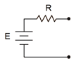
Figure 6.2.1 : Practical voltage source model.
The model for a voltage source adds a resistance in series, as shown in Figure 6.2.1 . This resistance sets an upper limit on the source's current output. Even if the output terminals are shorted, the maximum current will be dictated via Ohm's law to be the source voltage divided by the internal resistance, or \(E/R\). Obviously, this internal resistance will create some voltage divider effect with the attached load. To minimize this effect, the internal resistance should be as small as practicably possible. Thus,
\[\text{The ideal internal resistance of a voltage source is zero ohms (a short).} \nonumber \]
Given a zero ohm internal resistance, this improved model reverts back to the original ideal source. In the case of a lab power supply, the internal resistance typically will be a small fraction of an ohm.
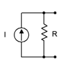
Figure 6.2.2 : Practical current source model.
For a current source, the improved model adds a resistance in parallel, as shown in Figure 6.2.2 . This resistance sets an upper limit on the source's voltage output. If the output terminals are opened, the maximum voltage will no longer produce a huge voltage. Instead, it is dictated by Ohm's law to be the source current times the internal resistance, or \(I \cdot R\). This internal resistance will create some current divider effect with the attached load. To minimize this effect, the internal resistance should be as large as practicably possible. Thus,
\[\text{The ideal internal resistance of a current source is infinite ohms.} \nonumber \]
Given an infinite ohm internal resistance (i.e., an open), this improved model reverts back to the original ideal source. From here on, whenever we deal with practical voltage and current sources, we understand that these sources have some associated internal resistance, even if they're not shown explicitly in a schematic diagram. Further, whenever we talk about ideal sources, we simply use a short for the internal resistance of a voltage source and an open for the internal resistance of a current source.
Source Equivalences
For any simple voltage source consisting of an ideal voltage source with a series internal resistance, an equivalent current source may be created. Similarly, for any simple current source consisting of an ideal current source with a parallel internal resistance, an equivalent voltage source may be created. By “equivalent”, we mean the load currents must be identical for both circuits given any value of load resistance. (Note that if the currents are the same then the voltages must also be the same due to Ohm’s Law.) Consider the simple voltage source of Figure 6.2.1 . Its equivalent current source would be that shown in Figure 6.2.2 . The opposite is also true.
For reasons that will become apparent under the section on Thévenin's theorem following, the internal resistances of these two circuits must be identical if they are to behave identically. Knowing that, it is a straightforward process to find the required value of the other source. As the current/voltage characteristic is linear for these circuits, a plot line can be defined by just two points. The two obvious points to use are the opened and shorted load cases. In other words, if it's equivalent for these two situations, it must work for any load. The shorted load case produces the maximum load current with zero load voltage, while in contrast, the opened load case produces the maximum load voltage with zero load current.
Given a voltage source, the maximum current is developed when the load is shorted producing a current of \(E/R\). Under that same load condition, all of the current from the current source version must be flowing through the load. Therefore, the value of the equivalent current source must be the maximum current of \(E/R\). It would be nonsensical to use a current source that was larger or smaller than this value.
To continue, if we look at the open load case, for the voltage source the load current would be zero and the load voltage would be the entire source voltage of \(E\). For the current source, the load would also see no current and its voltage would be the voltage appearing across its internal resistance which is \(R\) times the current \(E/R\), or just \(E\). Thus, the two behave identically at the load limits.
Similarly, if we start with a current source, an open load produces the maximum load voltage of \(I \cdot R\). Therefore, the equivalent voltage source must have a value of \(I \cdot R\). For the current source, a shorted load would produce a load current equal to the source value, or \(I\). The voltage source version would produce a current of \(E/R\), where the value of \(E\) was just found to be equal to \(I \cdot R\), and thus the load current would be \(I \cdot R/R\), or just \(I\). Once again, the two versions behave identically at the load limits.
To summarize the process of source conversion:
- The internal resistance will be the same for both versions.
- If converting from a voltage source to a current source, the value of the current source will be the maximum current available from the voltage source (shorted load case), and is equal to \(E/R\).
- If converting from a current source to a voltage source, the value of the voltage source will be the maximum voltage available from the current source (opened load case), and is equal to \(I \cdot R\).
If a multi-source is being converted (i.e., voltage sources in series or current sources in parallel), first combine the sources to arrive at the simplest source and then do the conversion. Do not convert the sources first and then combine them as you will wind up with series-parallel configurations rather than simple sources.
Judicious use of source conversions can sometimes simplify multi-source circuits by allowing converted sources to be combined, resulting in a single source.
Determine the current source equivalent for the source of Figure 6.2.3 .
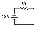
Figure 6.2.3 : Source for Example 6.2.1 .
First off, the resistance value is simply copied over, therefore the internal resistance of the current source is 50 \( \Omega \). The value of the current source is computed using Ohm's law based on the maximum current produced under the shorted load case. Thus, all 15 volts drops across the 50 \( \Omega \) resistance.
\[I_s = \frac{E}{R_s} \nonumber \]
\[I_s = \frac{15V}{50 \Omega} \nonumber \]
\[I_s = 0.3A \nonumber \]
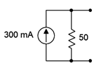
Figure 6.2.4 : Equivalent current source for the source of Figure 6.2.3 .
The equivalent current source is shown in Figure 6.2.4 . We know that this will work for the shorted an opened cases, but if any doubt is left as to its universal nature, simply substitute any other resistance value and compare the outcomes of the two circuits. For no particular reason, let's try using a load of 200 \( \Omega \) and see if the load currents are identical.
For the original voltage source we can use Ohm's law:
\[I_L = \frac{E}{R_s+R_L} \nonumber \]
\[I_L = \frac{15 V}{50 \Omega +200 \Omega} \nonumber \]
\[I_L = 60 mA \nonumber \]
For the equivalent current source we can use CDR:
\[I_L = I_s \frac{R_s}{R_s+R_L} \nonumber \]
\[I_L = 0.3 A \frac{50 \Omega}{50 \Omega +200 \Omega} \nonumber \]
\[I_L = 60 mA \nonumber \]
Try this with any other load resistor. The results should always be identical.
Now let's try one going the other way.
Determine the voltage source equivalent for the source of Figure 6.2.5 .
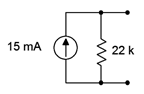
Figure 6.2.5 : Source for Example 6.2.2 .
Once again, the resistance value is simply copied over, therefore the internal resistance of the voltage source is 22 k\( \Omega \). The value of the voltage source is based on the maximum voltage produced under the opened load case and is computed using Ohm's law. For the open case, all 15 milliamps flows through the 22 k\( \Omega \) resistance.
\[E_s = I \times Rs \nonumber \]
\[E_s = 15 mA \times 22k \Omega \nonumber \]
\[E_s = 330 V \nonumber \]
The equivalent voltage source is shown in Figure 6.2.6 . Again, let's try using another value of load resistor to see if the load current and voltage results are identical between the two sources. This time, we'll match the load to the internal resistance of 22 k\( \Omega \).
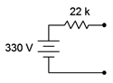
Figure 6.2.6 : Equivalent current source for the source of Figure 6.2.5 .
For a voltage source with matched resistances we wind up with a simple 50% voltage divider, thus the load voltage will be half the source voltage, or 165 volts. The original current source sees the current split in half due to the current divider rule. Thus, the load current should be 7.5 mA. Given this current, the load voltage will be,
\[V_L = I \times Rs \nonumber \]
\[V_L = 7.5mA \times 22 k \Omega \nonumber \]
\[V_L = 165 V \nonumber \]
Once again the results turn out to be identical.
Now that we have it is possible to substitute one kind of source for another, it is time to investigate how we might put this to use beyond just giving us a different way of driving a circuit. If applied intelligently, source conversions can be used to simplify and reduce complex circuits, and thus ease computational difficulty. For example, consider the circuit of Figure 6.2.7 .
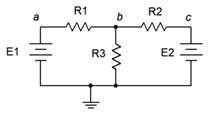
Figure 6.2.7 : A dual source circuit.
This circuit is unlike any circuit we have seen so far. Although we have analyzed circuits using multiple voltage sources, they have always been in a simple series loop. As such, their voltages may be added together to find a single equivalent voltage source. Such is not the case here. In this circuit the voltage sources are part of a series-parallel network and thus their potentials cannot be merely added. In fact, there are no further simplifications to be performed on this circuit using basic series-parallel techniques. We appear to be stuck.
But we're not. This circuit can be simplified into a straight all-parallel network through the use of source conversions. The \(E_1\), \(R_1\) combo can be converted into one current source while the \(E_2\), \(R_2\) combo can be converted into a second source. Once these are converted, the resulting circuit will consist of two current sources and three resistors, all in parallel. This is the sort of circuit we solved back in Chapter 4.
Determine \(V_b\) for the circuit of Figure 6.2.8 .
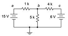
Figure 6.2.8 : Circuit for Example 6.2.3 .
The first step will be to convert the voltage sources into current sources. We will treat the resistors attached to their positive terminals as their internal resistances. In other words, we have a 15 volt source with 1 k\( \Omega \) resistance and a 6 volt source with a 4 k\( \Omega \) resistance.
For the first source, the current will be:
\[I_s = \frac{E}{R_s} \nonumber \]
\[I_s = \frac{15 V}{1k \Omega} \nonumber \]
\[I_s = 15mA \nonumber \]
And for the second source:
\[I_s = \frac{E}{R_s} \nonumber \]
\[I_s = \frac{6V}{4 k \Omega} \nonumber \]
\[I_s = 1.5mA \nonumber \]
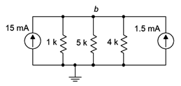
Figure 6.2.9 : Equivalent current source version of the circuit depicted in Figure 6.2.8 .
The equivalent converted circuit is shown in Figure 6.2.9 . Before continuing, it is worth noting that connection nodes \(a\) and \(c\) no longer exist in this circuit. More on this in a moment. This new circuit consists of a pair of current sources that sum to 16.5 mA and which drive three parallel resistors, 1 k\( \Omega \) \(||\) 4 k\( \Omega \) \(||\) 5 k\( \Omega \), or approximately 689.7 \( \Omega \). Ohm's law tells us \(V_b\) is:
\[V_b = I_{Total} \times R_{Equivalent} \nonumber \]
\[V_b \approx 16.5mA \times 689.7 \Omega \nonumber \]
\[V_b = 11.38V \nonumber \]
We can now take this voltage and apply it back into the original (unconverted) circuit. With this potential known, it is relatively easy to determine the other currents and voltages using KVL and Ohm's law. Looking at the 1 k\( \Omega \) resistor, the voltage across it must be 15 V − 11.38 V, or 3.62 V. Therefore, the current through it must be 3.62 mA. Similarly, the voltage across the 4 k\( \Omega \) resistor must be 11.38 V − 6 V, or 5.38 V, which yields a current of 1.345 mA. Both of these currents are flowing left to right. Then third current, flowing down through the 5 k\( \Omega \), is 11.38 V/5 k\( \Omega \), or 2.276 mA. KCL states that the current entering node \(b\) must equal the currents leaving. The entering current is 3.62 mA. The exiting currents are 1.345 mA and 2.276 mA, or 3.62 mA when rounded to three places (like the entering current).
As mentioned, nodes \(a\) and \(c\) disappeared in the converted circuit in Example 6.2.3 . This brings up an important point. Equivalent circuits are equivalent in terms that the items connected to the equivalent behave the same way as they do with the original circuit. That does not mean that the items within the equivalent see the same current or voltage. We do not expect the voltage across the 1 k\( \Omega \) or 4 k\( \Omega \) resistors in the converted version to be the same as those in the original version.