Analog computers are used to simulate physical systems. These systems may be electrical, mechanical, acoustical, or what have you. An analog computer is basically a collection of integrators, differentiators, summers, and amplifiers. Due to their relative stability, integrators are favored over differentiators. It is not uncommon for analog computers to be made without any differentiators. Because physical systems may be described in terms of differential equations, analog computers may be used to solve these equations, thus producing as output some system parameter.
The basic advantage of simulation is that several variations of a given system may be examined in real time without actually constructing the system. For a large project this is particularly cost-efficient. The process starts by writing a differential Equation (first-, second-, or third-order) that describes the system in question. The Equation is then solved for its highest-order element, and the result used to create a circuit.
Example \(\PageIndex{1}\)
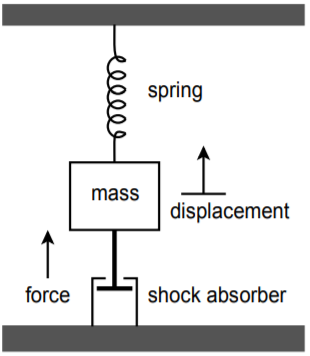
Let's investigate the system shown in Figure \(\PageIndex{1}\). This is a simple mechanical system that might represent (to a rough approximation) a variety of physical entities, including the suspension of an automobile.

Figure \(\PageIndex{1}\): Mechanical system.
This system is comprised of a body with mass \(M\), that is suspended from a spring. The spring has a spring constant, \(K\). The mass is also connected to a shock absorber that produces damping, \(R\). If an external force, \(F\), excites the mass, it will move, producing some displacement, \(X\). This displacement depends on the mass, force, spring constant, and damping. Essentially, the spring and shock absorber will create reactionary forces. From basic physics, \(F = MA\), where \(A\) is the acceleration of the body. If \(X\) is the position of the body, then \(dX/dt\) is its velocity, and \(d^2X/dt^2\) is its acceleration. Therefore, we can say
\[F = M \frac{d^2 X}{dt^2} \nonumber \]
In this system, the total force is comprised of the excitation force \(F\), and the forces produced by the spring and shock absorber.
\[F − F_{spring} − F_{shock} = M \frac{d^2 X}{dt^2} \nonumber \]
The spring's force is equal to the displacement times the spring constant:
\[F_{spring} = KX \nonumber \]
The shock absorber's force is equal to the damping constant times the velocity of the body:
\[F_{shock} = R \frac{dX}{dt} \nonumber \]
By substituting and rearranging the above elements we find that
\[F = M \frac{d^2 X} {dt^2} +R \frac{dX}{dt} +K X \nonumber \]
Here \(F\) is seen as the input signal, and \(X\) as the output signal. A somewhat less busy notation form is the dot convention. A single dot represents the first derivative with respect to time, two dots represent the second derivative, and so on. The above Equation may be rewritten as
\[F = M \ddot{X} +R \dot{X} +K X \nonumber \]
This is the final differential equation. Note how it contains only derivatives and no integrals. The last step is to solve the Equation for the highest-order differential. By setting it up in this form, the simulation circuit may be realized without using differentiators. This will indicate how many integrators will be required.
\[\ddot{X} = \frac{F}{M} − \frac{R}{M} \dot{X} − \frac{K}{M} X \nonumber \]
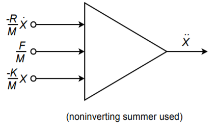
This says that the second differential of \(X\) is the sum of three components. To realize the circuit, start with a summing amplifier with the three desired signals as inputs. This is shown in block form in Figure \(\PageIndex{2}\). Note that two of the inputs use \(X\) and the first derivative of \(X\).

Figure \(\PageIndex{2}\): Circuit realization (block form).
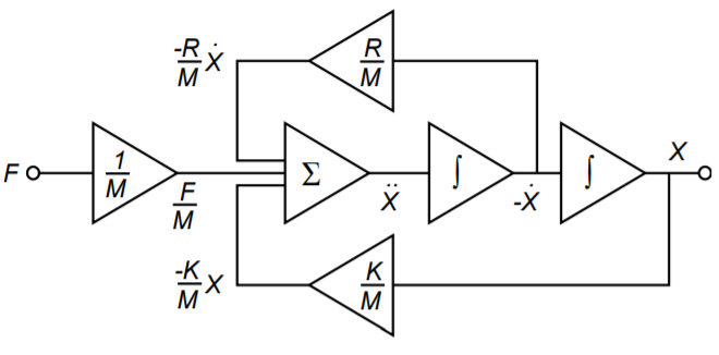
These elements may be produced by integrating the output of Figure \(\PageIndex{2}\). Appropriate constants may be used to achieve the desired signal levels. This is shown in Figure \(\PageIndex{3}\). Certain elements may be combined; for example, a weighted summing amplifier may be used to eliminate unneeded amplifiers.

Figure \(\PageIndex{3}\): Circuit realization using function blocks.
In use, the constants \(R\), \(K\), and \(M\) are set by potentiometers (they are essentially nothing more than scaled gain factors). A voltage representing the excitation force is applied to the circuit, and the desired output quantity is recorded. Note that the output of interest could be the acceleration, velocity, or displacement of the body. In order to test the system with a new spring or damping constant, all that is needed is to adjust the appropriate potentiometer. In this manner, a large number of combinations may be tried quickly. The most successful combinations may then be built and tested for the final design. An analog computer such as this would be very useful in testing such items as the suspension of an automobile or a loudspeaker system. To ease the design of the simulation circuit, commercial analog computers are available. Construction (or programming) of the circuit involves wiring integrator, amplifier, and summer blocks, together with the appropriate potentiometers. In this way, the details of designing and optimizing individual integrators or amplifiers is bypassed.


