7.11.6: Extended Topic- Other Integrator and Differentiator Circuits

Last updated
Save as PDF

Page ID: 53020

\( \newcommand{\vecs}[1]{\overset { \scriptstyle \rightharpoonup} {\mathbf{#1}} } \) \( \newcommand{\vecd}[1]{\overset{-\!-\!\rightharpoonup}{\vphantom{a}\smash {#1}}} \)\(\newcommand{\id}{\mathrm{id}}\) \( \newcommand{\Span}{\mathrm{span}}\) \( \newcommand{\kernel}{\mathrm{null}\,}\) \( \newcommand{\range}{\mathrm{range}\,}\) \( \newcommand{\RealPart}{\mathrm{Re}}\) \( \newcommand{\ImaginaryPart}{\mathrm{Im}}\) \( \newcommand{\Argument}{\mathrm{Arg}}\) \( \newcommand{\norm}[1]{\| #1 \|}\) \( \newcommand{\inner}[2]{\langle #1, #2 \rangle}\) \( \newcommand{\Span}{\mathrm{span}}\) \(\newcommand{\id}{\mathrm{id}}\) \( \newcommand{\Span}{\mathrm{span}}\) \( \newcommand{\kernel}{\mathrm{null}\,}\) \( \newcommand{\range}{\mathrm{range}\,}\) \( \newcommand{\RealPart}{\mathrm{Re}}\) \( \newcommand{\ImaginaryPart}{\mathrm{Im}}\) \( \newcommand{\Argument}{\mathrm{Arg}}\) \( \newcommand{\norm}[1]{\| #1 \|}\) \( \newcommand{\inner}[2]{\langle #1, #2 \rangle}\) \( \newcommand{\Span}{\mathrm{span}}\)\(\newcommand{\AA}{\unicode[.8,0]{x212B}}\)

The basic integrator and differentiator circuits examined earlier may be extended into other forms. Perhaps the most obvious extension is to add multiple inputs, as in an ordinary summing amplifier. In complex systems, this concept may save the use of several op amps. A summing integrator is shown in Figure \(\PageIndex{1}\). Note its similarity to a normal summing amplifier. In this circuit, the input currents are summed at the inverting input of the op amp.

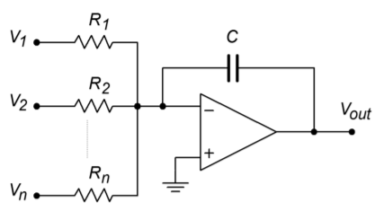
Figure \(\PageIndex{1}\): Summing integrator.

If the resistors are all set to the same value, we can quickly derive the output Equation by following the original derivation. The result is

\[V_{out} = − \frac{1}{RC} \int V_1 + V_2 + \dots + V_n dt \nonumber \]

The output is the negative integral of the sum of the inputs.

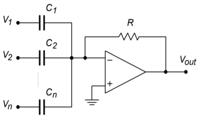
Figure \(\PageIndex{2}\): Summing differentiator.

In a similar vein, a summing differentiator may be formed. This is shown in Figure \(\PageIndex{2}\). Again, the proof of its output Equation follows the original differentiator derivation.

\[V_{out} = −RC_1 \frac{dV_1}{dt} −RC_2 \frac{dV_2}{dt} − \dots −RC_n \frac{dV_n}{dt} \nonumber \]

Another interesting adaptation of the integrator is the augmenting integrator. This circuit adds a constant gain portion to the output equation. An augmenting integrator is shown in Figure \(\PageIndex{3}\). The addition of the feedback resistor \(R_f\) provides the augmenting action. As you might surmise, the gain portion is directly related to \(R_f\) and \(R_i\).

\[V_{out} = −V_{in} \frac{R_f}{R_i} − \frac{1}{RC} \int V_{in} dt \nonumber \]

The augmenting integrator can also be turned into a summing/augmenting integrator by adding extra input resistors as in Figure \(\PageIndex{1}\). Note that the gain portion will be the same for all inputs if the input summing resistors are of equal value.

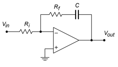
Figure \(\PageIndex{3}\): Augmenting integrator.

The final variant that we shall note is the double integrator. This design requires two reactive portions in order to achieve double integration. One possibility is shown in Figure \(\PageIndex{4}\). In this circuit, a pair of \(RC\) “Tee” networks are used. The output Equation is

\[V_{out} = − \frac{4}{(RC)^2} \int \int V_{in} dt \nonumber \]

When properly used, the double integrator can cut down the parts requirement of larger circuit designs.

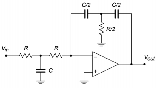
Figure \(\PageIndex{4}\): Double integrator.