10.3: Series Impedance
- Page ID
- 52955

\( \newcommand{\vecs}[1]{\overset { \scriptstyle \rightharpoonup} {\mathbf{#1}} } \)
\( \newcommand{\vecd}[1]{\overset{-\!-\!\rightharpoonup}{\vphantom{a}\smash {#1}}} \)
\( \newcommand{\dsum}{\displaystyle\sum\limits} \)
\( \newcommand{\dint}{\displaystyle\int\limits} \)
\( \newcommand{\dlim}{\displaystyle\lim\limits} \)
\( \newcommand{\id}{\mathrm{id}}\) \( \newcommand{\Span}{\mathrm{span}}\)
( \newcommand{\kernel}{\mathrm{null}\,}\) \( \newcommand{\range}{\mathrm{range}\,}\)
\( \newcommand{\RealPart}{\mathrm{Re}}\) \( \newcommand{\ImaginaryPart}{\mathrm{Im}}\)
\( \newcommand{\Argument}{\mathrm{Arg}}\) \( \newcommand{\norm}[1]{\| #1 \|}\)
\( \newcommand{\inner}[2]{\langle #1, #2 \rangle}\)
\( \newcommand{\Span}{\mathrm{span}}\)
\( \newcommand{\id}{\mathrm{id}}\)
\( \newcommand{\Span}{\mathrm{span}}\)
\( \newcommand{\kernel}{\mathrm{null}\,}\)
\( \newcommand{\range}{\mathrm{range}\,}\)
\( \newcommand{\RealPart}{\mathrm{Re}}\)
\( \newcommand{\ImaginaryPart}{\mathrm{Im}}\)
\( \newcommand{\Argument}{\mathrm{Arg}}\)
\( \newcommand{\norm}[1]{\| #1 \|}\)
\( \newcommand{\inner}[2]{\langle #1, #2 \rangle}\)
\( \newcommand{\Span}{\mathrm{span}}\) \( \newcommand{\AA}{\unicode[.8,0]{x212B}}\)
\( \newcommand{\vectorA}[1]{\vec{#1}} % arrow\)
\( \newcommand{\vectorAt}[1]{\vec{\text{#1}}} % arrow\)
\( \newcommand{\vectorB}[1]{\overset { \scriptstyle \rightharpoonup} {\mathbf{#1}} } \)
\( \newcommand{\vectorC}[1]{\textbf{#1}} \)
\( \newcommand{\vectorD}[1]{\overrightarrow{#1}} \)
\( \newcommand{\vectorDt}[1]{\overrightarrow{\text{#1}}} \)
\( \newcommand{\vectE}[1]{\overset{-\!-\!\rightharpoonup}{\vphantom{a}\smash{\mathbf {#1}}}} \)
\( \newcommand{\vecs}[1]{\overset { \scriptstyle \rightharpoonup} {\mathbf{#1}} } \)
\(\newcommand{\longvect}{\overrightarrow}\)
\( \newcommand{\vecd}[1]{\overset{-\!-\!\rightharpoonup}{\vphantom{a}\smash {#1}}} \)
\(\newcommand{\avec}{\mathbf a}\) \(\newcommand{\bvec}{\mathbf b}\) \(\newcommand{\cvec}{\mathbf c}\) \(\newcommand{\dvec}{\mathbf d}\) \(\newcommand{\dtil}{\widetilde{\mathbf d}}\) \(\newcommand{\evec}{\mathbf e}\) \(\newcommand{\fvec}{\mathbf f}\) \(\newcommand{\nvec}{\mathbf n}\) \(\newcommand{\pvec}{\mathbf p}\) \(\newcommand{\qvec}{\mathbf q}\) \(\newcommand{\svec}{\mathbf s}\) \(\newcommand{\tvec}{\mathbf t}\) \(\newcommand{\uvec}{\mathbf u}\) \(\newcommand{\vvec}{\mathbf v}\) \(\newcommand{\wvec}{\mathbf w}\) \(\newcommand{\xvec}{\mathbf x}\) \(\newcommand{\yvec}{\mathbf y}\) \(\newcommand{\zvec}{\mathbf z}\) \(\newcommand{\rvec}{\mathbf r}\) \(\newcommand{\mvec}{\mathbf m}\) \(\newcommand{\zerovec}{\mathbf 0}\) \(\newcommand{\onevec}{\mathbf 1}\) \(\newcommand{\real}{\mathbb R}\) \(\newcommand{\twovec}[2]{\left[\begin{array}{r}#1 \\ #2 \end{array}\right]}\) \(\newcommand{\ctwovec}[2]{\left[\begin{array}{c}#1 \\ #2 \end{array}\right]}\) \(\newcommand{\threevec}[3]{\left[\begin{array}{r}#1 \\ #2 \\ #3 \end{array}\right]}\) \(\newcommand{\cthreevec}[3]{\left[\begin{array}{c}#1 \\ #2 \\ #3 \end{array}\right]}\) \(\newcommand{\fourvec}[4]{\left[\begin{array}{r}#1 \\ #2 \\ #3 \\ #4 \end{array}\right]}\) \(\newcommand{\cfourvec}[4]{\left[\begin{array}{c}#1 \\ #2 \\ #3 \\ #4 \end{array}\right]}\) \(\newcommand{\fivevec}[5]{\left[\begin{array}{r}#1 \\ #2 \\ #3 \\ #4 \\ #5 \\ \end{array}\right]}\) \(\newcommand{\cfivevec}[5]{\left[\begin{array}{c}#1 \\ #2 \\ #3 \\ #4 \\ #5 \\ \end{array}\right]}\) \(\newcommand{\mattwo}[4]{\left[\begin{array}{rr}#1 \amp #2 \\ #3 \amp #4 \\ \end{array}\right]}\) \(\newcommand{\laspan}[1]{\text{Span}\{#1\}}\) \(\newcommand{\bcal}{\cal B}\) \(\newcommand{\ccal}{\cal C}\) \(\newcommand{\scal}{\cal S}\) \(\newcommand{\wcal}{\cal W}\) \(\newcommand{\ecal}{\cal E}\) \(\newcommand{\coords}[2]{\left\{#1\right\}_{#2}}\) \(\newcommand{\gray}[1]{\color{gray}{#1}}\) \(\newcommand{\lgray}[1]{\color{lightgray}{#1}}\) \(\newcommand{\rank}{\operatorname{rank}}\) \(\newcommand{\row}{\text{Row}}\) \(\newcommand{\col}{\text{Col}}\) \(\renewcommand{\row}{\text{Row}}\) \(\newcommand{\nul}{\text{Nul}}\) \(\newcommand{\var}{\text{Var}}\) \(\newcommand{\corr}{\text{corr}}\) \(\newcommand{\len}[1]{\left|#1\right|}\) \(\newcommand{\bbar}{\overline{\bvec}}\) \(\newcommand{\bhat}{\widehat{\bvec}}\) \(\newcommand{\bperp}{\bvec^\perp}\) \(\newcommand{\xhat}{\widehat{\xvec}}\) \(\newcommand{\vhat}{\widehat{\vvec}}\) \(\newcommand{\uhat}{\widehat{\uvec}}\) \(\newcommand{\what}{\widehat{\wvec}}\) \(\newcommand{\Sighat}{\widehat{\Sigma}}\) \(\newcommand{\lt}{<}\) \(\newcommand{\gt}{>}\) \(\newcommand{\amp}{&}\) \(\definecolor{fillinmathshade}{gray}{0.9}\)Perhaps the first practical issue we face is determining the effective impedance of an RLC series loop. For starters, resistors in series simply add. Reactances also add but we must be careful of the sign. Inductive reactance and capacitive reactance will partially cancel each other. Thus, the impedance in rectangular form is the sum of the resistive components for the real portion, plus the sum of the reactances for the imaginary (\(j\)) portion. We will often find it convenient to express this value in polar form.
Example \(\PageIndex{1}\)
What is the impedance of the network shown in Figure \(\PageIndex{1}\) at a frequency of 15 kHz?
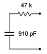
First we need to find the capacitive reactance value.
\[X_C = − j \frac{1}{2\pi f C} \nonumber \]
\[X_C = − j \frac{1}{2\pi 15kHz 910 pF} \nonumber \]
\[X_C = − j 11.66 k \Omega \nonumber \]
As there is only one resistor and one capacitor, the result in rectangular form is \(47 k −j11.66 k\Omega\). In polar form this is:
\[\text{Magnitude } = \sqrt{\text{Real}^2+\text{Imaginary}^2} \nonumber \]
\[\text{Magnitude } = \sqrt{47k^2+(−11.66 k)^2} \nonumber \]
\[\text{Magnitude } = 48.42 k \nonumber \]
\[\theta = \tan^{−1} \left( \frac{\text{Imaginary}}{\text{Real}} \right) \nonumber \]
\[\theta = \ tan^{−1} \left( \frac{−11.66 k}{47 k} \right) \nonumber \]
\[\theta = −13.9^{\circ}\nonumber \]
That is, in polar form \(Z = 48.42E3\angle −13.9^{\circ} \Omega\).
Example \(\PageIndex{2}\)
Determine the effective impedance of the circuit shown in Figure \(\PageIndex{2}\) if the source frequency is 2 kHz. Repeat this for source frequencies of 200 Hz and 20 kHz. Finally, express the results in both rectangular and polar form.
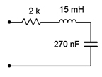
The first step is to find the reactance values at 2 kHz.
\[X_L = j 2\pi f L \nonumber \]
\[X_L = j 2\pi 2000Hz 15mH \nonumber \]
\[X_L = j 188.5 \Omega \nonumber \]
\[X_C = − j \frac{1}{2\pi f C} \nonumber \]
\[X_C = − j \frac{1}{2\pi 2000 Hz 270 nF} \nonumber \]
\[X_C = − j 294.7 \Omega \nonumber \]
Combine reals with reals and \(j\) terms with \(j\) terms.
\[Z = R+ j X_L − j X_C \nonumber \]
\[Z = 500+ j 188.5 − j 294.7 \Omega \nonumber \]
\[Z \approx 500− j 106.2\Omega = 511.2\angle −12^{\circ} \Omega \nonumber \]
At 200 Hz \(X_C\) will ten times larger and \(X_L\) will be ten times smaller.
\[X_C = −j2947 \Omega \nonumber \]
\[X_L = j18.85 \Omega \nonumber \]
\[Z = 500 + j18.85 −j2947 \Omega \nonumber \]
\[Z \approx 500 −j2928 \Omega = 2970\angle −80.3^{\circ} \Omega \nonumber \]
At 20 kHz \(X_C\) will ten times smaller and \(X_L\) will be ten times larger.
\[X_C = −j29.47 \Omega \nonumber \]
\[X_L = j1885 \Omega \nonumber \]
\[Z = 500 + j1885 −j29.47 \Omega \nonumber \]
\[Z \approx 500 + j1856 \Omega = 1922\angle 74.9^{\circ} \Omega \nonumber \]
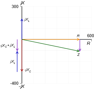
To help visualize this complex impedance, it is useful to construct a phasor plot as shown in Figure \(\PageIndex{3}\). We will do this for the initial case of 2 kHz. The resistive component is the horizontal vector of length 500 (yellow). \(X_L\) is straight up (blue) at \(188.5\angle 90^{\circ}\), and \(X_C\) is straight down (red) at \(294.7\angle −90^{\circ}\). By copying the \(X_L\) vector and then shifting it down and next to \(X_C\), the difference between the two reactive components can be seen (purple component directly above the \(X_L\) copy). This Figure \(\PageIndex{2}\) Circuit for Example \(\PageIndex{2}\). reactive sum is then copied and shifted right to join the resistive component to show the final result. This is \(511.2\angle −12^{\circ} \Omega\) (green), as expected.
Example \(\PageIndex{3}\)
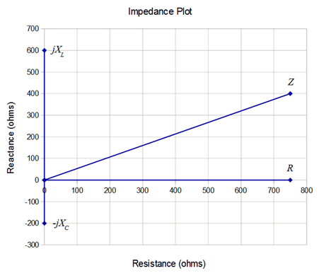
Determine the impedance of the network shown in Figure \(\PageIndex{4}\). If the input frequency is 1 kHz, determine the capacitor and inductor values.
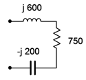
The reactance values are already given, so we simply add them to determine the impedance in rectangular form. Combine reals with reals and \(j\) terms with \(j\) terms, and then convert to polar form.
\[Z = R+j X_L − j X_C \nonumber \]
\[Z = 750+j 600 − j 200 \Omega \nonumber \]
\[Z = 750+j 400 \Omega = 850\angle 28.1^{\circ} \Omega \nonumber \]
To find the capacitance and inductance, we simply rearrange the reactance formulas and solve. First, the inductor:
\[X_L = j 2\pi f L \nonumber \]
\[L = \frac{| X_L |}{2\pi f} \nonumber \]
\[L = \frac{ 600\Omega}{2\pi 1kHz} \nonumber \]
\[L \approx 95.5 mH \nonumber \]
And now for the capacitor:
\[X_C = − j \frac{1}{2 \pi f C} \nonumber \]
\[C = \frac{1}{2\pi f | X_C | } \nonumber \]
\[C = \frac{1}{2\pi 1 kHz 200 \Omega} \nonumber \]
\[C = 796 nF \nonumber \]
A plot of the impedance vector summation is shown in Figure \(\PageIndex{5}\). Note how the three components combine graphically to arrive at \(Z\).