
11.3: Parallel Impedance
- Page ID
- 52963

\( \newcommand{\vecs}[1]{\overset { \scriptstyle \rightharpoonup} {\mathbf{#1}} } \)
\( \newcommand{\vecd}[1]{\overset{-\!-\!\rightharpoonup}{\vphantom{a}\smash {#1}}} \)
\( \newcommand{\dsum}{\displaystyle\sum\limits} \)
\( \newcommand{\dint}{\displaystyle\int\limits} \)
\( \newcommand{\dlim}{\displaystyle\lim\limits} \)
\( \newcommand{\id}{\mathrm{id}}\) \( \newcommand{\Span}{\mathrm{span}}\)
( \newcommand{\kernel}{\mathrm{null}\,}\) \( \newcommand{\range}{\mathrm{range}\,}\)
\( \newcommand{\RealPart}{\mathrm{Re}}\) \( \newcommand{\ImaginaryPart}{\mathrm{Im}}\)
\( \newcommand{\Argument}{\mathrm{Arg}}\) \( \newcommand{\norm}[1]{\| #1 \|}\)
\( \newcommand{\inner}[2]{\langle #1, #2 \rangle}\)
\( \newcommand{\Span}{\mathrm{span}}\)
\( \newcommand{\id}{\mathrm{id}}\)
\( \newcommand{\Span}{\mathrm{span}}\)
\( \newcommand{\kernel}{\mathrm{null}\,}\)
\( \newcommand{\range}{\mathrm{range}\,}\)
\( \newcommand{\RealPart}{\mathrm{Re}}\)
\( \newcommand{\ImaginaryPart}{\mathrm{Im}}\)
\( \newcommand{\Argument}{\mathrm{Arg}}\)
\( \newcommand{\norm}[1]{\| #1 \|}\)
\( \newcommand{\inner}[2]{\langle #1, #2 \rangle}\)
\( \newcommand{\Span}{\mathrm{span}}\) \( \newcommand{\AA}{\unicode[.8,0]{x212B}}\)
\( \newcommand{\vectorA}[1]{\vec{#1}} % arrow\)
\( \newcommand{\vectorAt}[1]{\vec{\text{#1}}} % arrow\)
\( \newcommand{\vectorB}[1]{\overset { \scriptstyle \rightharpoonup} {\mathbf{#1}} } \)
\( \newcommand{\vectorC}[1]{\textbf{#1}} \)
\( \newcommand{\vectorD}[1]{\overrightarrow{#1}} \)
\( \newcommand{\vectorDt}[1]{\overrightarrow{\text{#1}}} \)
\( \newcommand{\vectE}[1]{\overset{-\!-\!\rightharpoonup}{\vphantom{a}\smash{\mathbf {#1}}}} \)
\( \newcommand{\vecs}[1]{\overset { \scriptstyle \rightharpoonup} {\mathbf{#1}} } \)
\(\newcommand{\longvect}{\overrightarrow}\)
\( \newcommand{\vecd}[1]{\overset{-\!-\!\rightharpoonup}{\vphantom{a}\smash {#1}}} \)
\(\newcommand{\avec}{\mathbf a}\) \(\newcommand{\bvec}{\mathbf b}\) \(\newcommand{\cvec}{\mathbf c}\) \(\newcommand{\dvec}{\mathbf d}\) \(\newcommand{\dtil}{\widetilde{\mathbf d}}\) \(\newcommand{\evec}{\mathbf e}\) \(\newcommand{\fvec}{\mathbf f}\) \(\newcommand{\nvec}{\mathbf n}\) \(\newcommand{\pvec}{\mathbf p}\) \(\newcommand{\qvec}{\mathbf q}\) \(\newcommand{\svec}{\mathbf s}\) \(\newcommand{\tvec}{\mathbf t}\) \(\newcommand{\uvec}{\mathbf u}\) \(\newcommand{\vvec}{\mathbf v}\) \(\newcommand{\wvec}{\mathbf w}\) \(\newcommand{\xvec}{\mathbf x}\) \(\newcommand{\yvec}{\mathbf y}\) \(\newcommand{\zvec}{\mathbf z}\) \(\newcommand{\rvec}{\mathbf r}\) \(\newcommand{\mvec}{\mathbf m}\) \(\newcommand{\zerovec}{\mathbf 0}\) \(\newcommand{\onevec}{\mathbf 1}\) \(\newcommand{\real}{\mathbb R}\) \(\newcommand{\twovec}[2]{\left[\begin{array}{r}#1 \\ #2 \end{array}\right]}\) \(\newcommand{\ctwovec}[2]{\left[\begin{array}{c}#1 \\ #2 \end{array}\right]}\) \(\newcommand{\threevec}[3]{\left[\begin{array}{r}#1 \\ #2 \\ #3 \end{array}\right]}\) \(\newcommand{\cthreevec}[3]{\left[\begin{array}{c}#1 \\ #2 \\ #3 \end{array}\right]}\) \(\newcommand{\fourvec}[4]{\left[\begin{array}{r}#1 \\ #2 \\ #3 \\ #4 \end{array}\right]}\) \(\newcommand{\cfourvec}[4]{\left[\begin{array}{c}#1 \\ #2 \\ #3 \\ #4 \end{array}\right]}\) \(\newcommand{\fivevec}[5]{\left[\begin{array}{r}#1 \\ #2 \\ #3 \\ #4 \\ #5 \\ \end{array}\right]}\) \(\newcommand{\cfivevec}[5]{\left[\begin{array}{c}#1 \\ #2 \\ #3 \\ #4 \\ #5 \\ \end{array}\right]}\) \(\newcommand{\mattwo}[4]{\left[\begin{array}{rr}#1 \amp #2 \\ #3 \amp #4 \\ \end{array}\right]}\) \(\newcommand{\laspan}[1]{\text{Span}\{#1\}}\) \(\newcommand{\bcal}{\cal B}\) \(\newcommand{\ccal}{\cal C}\) \(\newcommand{\scal}{\cal S}\) \(\newcommand{\wcal}{\cal W}\) \(\newcommand{\ecal}{\cal E}\) \(\newcommand{\coords}[2]{\left\{#1\right\}_{#2}}\) \(\newcommand{\gray}[1]{\color{gray}{#1}}\) \(\newcommand{\lgray}[1]{\color{lightgray}{#1}}\) \(\newcommand{\rank}{\operatorname{rank}}\) \(\newcommand{\row}{\text{Row}}\) \(\newcommand{\col}{\text{Col}}\) \(\renewcommand{\row}{\text{Row}}\) \(\newcommand{\nul}{\text{Nul}}\) \(\newcommand{\var}{\text{Var}}\) \(\newcommand{\corr}{\text{corr}}\) \(\newcommand{\len}[1]{\left|#1\right|}\) \(\newcommand{\bbar}{\overline{\bvec}}\) \(\newcommand{\bhat}{\widehat{\bvec}}\) \(\newcommand{\bperp}{\bvec^\perp}\) \(\newcommand{\xhat}{\widehat{\xvec}}\) \(\newcommand{\vhat}{\widehat{\vvec}}\) \(\newcommand{\uhat}{\widehat{\uvec}}\) \(\newcommand{\what}{\widehat{\wvec}}\) \(\newcommand{\Sighat}{\widehat{\Sigma}}\) \(\newcommand{\lt}{<}\) \(\newcommand{\gt}{>}\) \(\newcommand{\amp}{&}\) \(\definecolor{fillinmathshade}{gray}{0.9}\)Perhaps the first order of business is to determine equivalent impedance values for some collection of parallel components. Recall that the reciprocal of reactance is susceptance,
\[S = \dfrac{1}{X} \label{3.2} \]
and that the reciprocal of impedance is admittance,
\[Y = \dfrac{1}{Z} \label{3.3} \]
The units are siemens for each. It is also worth noting that, due to the division, the signs reverse. For example, a capacitive susceptance has an angle of +90 degrees and if a complex admittance has a negative angle, then the associated impedance is inductive.
The “conductance rule” for parallel combinations studied in the DC case remains valid for the AC case, although we generalize it for impedances:
\[Z_{total} = \dfrac{1}{\dfrac{1}{Z_1} + \dfrac{1}{Z_2} + \dfrac{1}{Z_3} + \dots + \dfrac{1}{Z_N}} \label{3.4} \]
Each of the individual impedances presented in Equation \ref{3.4} (i.e., \(Z_1\), \(Z_2\), etc) can represent a simple resistance, a pure reactance or a complex impedance. Further, the product-sum rule shortcut for two components also remains valid for AC components:
\[Z_{total} = \dfrac{Z_1 \times Z_2}{Z_1+Z_2} \label{3.5} \]
There is one special case where Equation \ref{3.5} can be “troublesome”, and that's when the two impedances consist of a pure capacitive reactance and a pure inductive reactance, both of the same magnitude. The two items will effectively cancel each other leaving a denominator of zero and an undefined result. While the theoretical combination “blows up” and approaches infinity, in reality it is limited by associated resistances such as \(R_{coil}\), and arrives at some finite value This situation is studied in great depth in Chapter 8, which covers the concept of resonance.
Example \(\PageIndex{1}\)
Determine the impedance of the network shown in Figure \(\PageIndex{1}\).
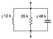
Equation \ref{3.4} would be best here.
\[Z_{total} = \dfrac{1}{\dfrac{1}{Z_1} + \dfrac{1}{Z_2} + \dfrac{1}{Z_3}} \nonumber \]
\[Z_{total} = \dfrac{1}{\dfrac{1}{j 12 k\Omega} + \dfrac{1}{20 k \Omega} + \dfrac{1}{− j 48 k\Omega}} \nonumber \]
\[Z_{total} = 12.49E3\angle 51.3^{\circ} \Omega \nonumber \]
This result might be a little surprising to the sharp-eyed. Notice that the magnitude of the total is larger than the magnitude of the smallest component (the inductor at \(j12 k\Omega\)). This would never be the case if these three components were all resistors: the result would have to be smaller than the smallest element in the group.
The reason for this is that the capacitive reactance partially cancels the inductive reactance. If the product-sum rule (Equation \ref{3.5}) is used with these two components, the result is \(16E3\angle 90^{\circ}\) or \(j16 k\Omega\). Placing that in parallel with the 20 k\(\Omega\) resistor (again using Equation \ref{3.5}) leads to the result computed above.
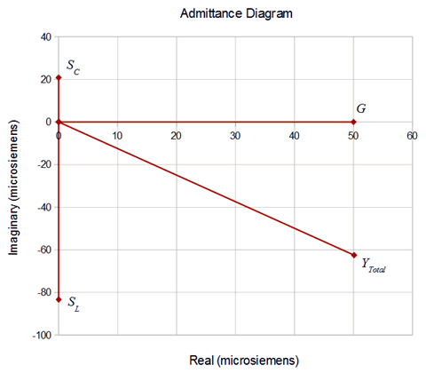
An admittance diagram is illustrated in Figure \(\PageIndex{2}\). The vector summation of the component conductance and susceptances is verified nicely.
The individual component values are:
\[S_L = \dfrac{1}{j 12k \Omega} \approx − j 83.33E-6S \nonumber \]
\[S_C = \dfrac{1}{− j 48k \Omega} \approx j 20.83E-6S \nonumber \]
\[G = \dfrac{1}{20 k\Omega} = 50E-6 S \nonumber \]
\[Y_{total} = \dfrac{1}{12.49E3\angle 51.3^{\circ} \Omega} \approx 80.1E-6\angle −51.3^{\circ} S \nonumber \]
In rectangular form \(Y_{total} = 50E−6 − j62.5E−6 S\).
Example \(\PageIndex{2}\)
Determine the impedance of the network shown in Figure \(\PageIndex{3}\) at a frequency of 10 kHz. Repeat this for a frequency of 1 kHz.
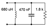
First, find the reactances at 10 kHz. For the inductor we find:
\[X_L = j 2\pi f L \nonumber \]
\[X_L = j 2\pi 10 kHz680 \mu H \nonumber \]
\[X_L \approx j 42.73\Omega \nonumber \]
And for the capacitor:
\[X_C = − j \dfrac{1}{2 \pi f C} \nonumber \]
\[X_C = − j \dfrac{1}{2 \pi 10kHz 470 nF} \nonumber \]
\[X_C \approx − j 33.86\Omega \nonumber \]
Now use Equation \ref{3.4} to combine the elements.
\[Z_{total} = \dfrac{1}{\dfrac{1}{Z_1} + \dfrac{1}{Z_2} + \dfrac{1}{Z_3}} \nonumber \]
\[Z_{total} = \dfrac{1}{\dfrac{1}{j 42.73\Omega} + \dfrac{1}{1.8k \Omega} + \dfrac{1}{− j 33.86\Omega}} \nonumber \]
\[Z_{total} = 162.6\angle −84.8^{\circ} \Omega \nonumber \]
In rectangular form this is \(14.68 − j161.9 \Omega\). As the capacitor's reactance is the smallest of the three components, it dominates the equivalent impedance at this frequency. By working the capacitive reactance formula in reverse, it can be shown that the reactive portion of \(− j161.9 \Omega\) can achieved at this frequency by using a capacitance of 98.3 nF. That means that at 10 kHz, this parallel network has the same impedance as a 14.68 \(\Omega\) resistor in series with a 98.3 nF capacitor. At any other frequency this will no longer be true, as will be illustrated momentarily.
At 1 kHz, the frequency is reduced by a factor of ten. Therefore, \(X_L\) will be ten times lower, or approximately \(j4.273 \Omega\). Further, \(X_C\) will be ten times higher, or about \(− j338.6 \Omega\). The inductive reactance will now dominate.
The new impedance is:
\[Z_{total} = \dfrac{1}{\dfrac{1}{Z_1} + \dfrac{1}{Z_2} + \dfrac{1}{Z_3}} \nonumber \]
\[Z_{total} = \dfrac{1}{\dfrac{1}{j 4.273\Omega} + \dfrac{1}{1.8k \Omega} + \dfrac{1}{− j 338.6\Omega}} \nonumber \]
\[Z_{total} = 4.328\angle 89.9^{\circ} \Omega \nonumber \]
In rectangular form this is \(10.4E−3 + j4.328 \Omega\). The result is inductive, the opposite of what we saw at 10 kHz. Using the inductive reactance formula, it can be shown that at 1 kHz this parallel network has the same impedance as a 10.4 milliohm resistor in series with a 689 \(\mu\)H inductor.